Internal data
Overview
This chapter explains how to obtain various data from simulation and how to plot them. Using per-simulation labels for things is exaplained, and scene tags are introduced.
Plotting
In the previous chapter, a simple simulation of a sphere falling onto the plane was created. The only output so far was the 3d view. Let’s see how we can plot some data, such as \(z(t)\), i.e. the evolution of the \(z\)-coordinate of the sphere over time. It consists of two separate tasks:
Collecting data to plot, since we need to keep history;
Saying how to plot which of the collected data.
Plot data are stored in S.plot.data, keyed by some unique name, in series (“rows”); data are always added to all “columns” (a Not a Number is automatically added to rows which are not defined at the time-point).
We can define what to plot by setting S.plot.plots. It is a dictionary, which is given in the form of {key:value,...}. The key is the \(x\)-axis data key, value is a tuple. Better give an example, in the following.
Simplified interface
With the simplified interface, expressions to be evaluated are used as plot keys directly:
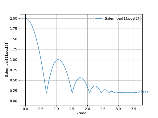
S.plot.plots={'S.time': ('S.dem.par[1].pos[2]',)}
This would plot \(z\)-position (pos[2], as pos is a vector in 3d) of the 1st particle (the sphere) against time. We need to add an engine which will save the data for us:
S.engines=S.engines+[PyRunner(10,'S.plot.autoData()')]
PyRunner runs an arbitrary python code every n steps; so we use previous-defined engines and add the PyRunner to it, which will call S.plot.autoData() every 10 steps. PyRunner automatically sets several variables which can be used inside expressions – one of them is S, the current scene (for which the engine is called).
from past.builtins import execfile
execfile('basic-1.py')                                  # re-use the simple setup for brevity
S.plot.plots={'S.time': ('S.dem.par[1].pos[2]',)}       # define what to plot
S.engines=S.engines+[PyRunner(10,'S.plot.autoData()')]  # add the engine
S.throttle=0                                            # run at full speed now
S.run(2000,True)                                        # run 2000 steps
S.plot.plot()                                           # show the plot
(Source code, png, hires.png, pdf)

Separate \(y\) axes
To make the plot prettier, \(x\)-axis and \(y\)-axis title can be set using the name=expression syntax. Multiple variables can be plotted on one \(y\)-axis; using None for key will put the rest on the \(y_2\) (right) \(y\)-axis. The following will plot \(z\) positions of both particles on the left and \(E_k\) (kinetic energy) of the sphere on the right:
S.plot.plots={'t=S.time': (     # complex expressions can span multiple lines in python :)
   '$z_1$=S.dem.par[1].pos[2]',
   '$z_0$=S.dem.par[0].pos[2]',
   None,                        # remaining things go to the y2 axis
   '$E_k$=S.dem.par[1].Ek'
)}
(Source code, png, hires.png, pdf)
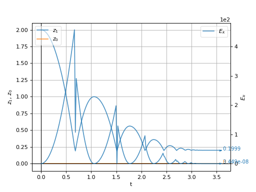
Note that we used math expressions $...$ for symbols in line labels; the syntax is very similar to LaTeX and is documented in detail in the underlying plotting library, Matplotlib.
Subfigures
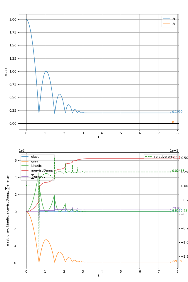
The S.plot.plots dictionary can contain multiple keys; each of them then creates a new sub-figure.
There is a limited support for specifying style of individual lines by using (key,format) instead of key, where format is Matlab-like syntax explained in detail here; it consists of color and line/marker abbreviation such as 'g--' specifying dashed green line.
This example also demonstrates that **expression denotes a dictionary-like object which contains values to be plotted (this syntax is similar to keyword argument syntax in Python); this feature is probably only useful with energy tracking where keys are not known a-priori.
We add another figure showing energies on the left; energy total (“\(\sum\) energy”) should be zero, as energy should be conserved, and relative error will be plotted on the right:
S.plot.plots={
   't=S.time':(
      '$z_1$=S.dem.par[1].pos[2]',
      '$z_0$=S.dem.par[0].pos[2]',
    ),
    ' t=S.time':(                                 # note the space before 't': explained below
      '**S.energy',                               # plot all energy fields on the first axis
      r'$\sum$ energy=S.energy.total()',          # compute total energy
      None,                                       # put the rest on the y2 axis
      ('relative error=S.energy.relErr()','g--')  # plot relative error of energy measures, dashed green
    )
}

# energy is not tracked by default, it must be turned on explicitly
S.trackEnergy=True
Note
We had to prepend space to the second \(x\)-axis in ” t=S.time”; otherwise, the second value would overwrite the first one, as dictionary must have unique keys. Spaces are stripped away, so they don’t appear in the output.
(Source code, png, hires.png, pdf)

Complex interface
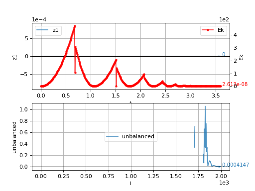
The complex interface requires one to assign keys to data using S.plot.addData. The advantage is that arbitrary computations can be performed on the data before they are stored. One usually creates a function to store the data in this way:
# use PyRunner to call our function periodically
S.engines=S.engines+[PyRunner(5,'myAddPlotData(S)')]
# define function which will be called by the PyRunner above
def myAddPlotData(S):
   ## do any computations here
   uf=woo.utils.unbalancedForce(S)
   ## store the data, use any keys you want
   S.plot.addData(t=S.time,i=S.step,z1=S.dem.par[1].pos[1],Ek=S.dem.par[1].Ek,unbalanced=uf)
# specify plots as usual
S.plot.plots={'t':('z1',None,('Ek','r.-')),'i':('unbalanced',)}
(Source code, png, hires.png, pdf)

Save plot data
Collected data can be saved to file using S.plot.saveDataTxt. This function creates (optionally compressed) text file with numbers written in columns; it can be readily loaded into NumPy via numpy.genfromtxt or into a spreadsheet program:
S.plot.saveDataTxt('basic-1.data.txt')
produces (only the beginning of the file is shown):
1 2 3 4 5 6 7 8 9 10 11 12 13 14 15 | # Ek i t unbalanced z1
0.0 0 0.0 nan 0.0
0.08358947705644633 5 0.009000000000000001 nan 0.0
0.3343579082257853 10 0.018 nan 0.0
0.7523052935080173 15 0.026999999999999996 nan 0.0
1.3374316329031413 20 0.036000000000000004 nan 0.0
2.0897369264111574 25 0.04500000000000002 nan 0.0
3.009221174032065 30 0.054000000000000034 nan 0.0
4.095884375765865 35 0.06300000000000004 nan 0.0
5.349726531612559 40 0.07200000000000002 nan 0.0
6.770747641572144 45 0.081 nan 0.0
8.35894770564462 50 0.08999999999999998 nan 0.0
10.11432672382999 55 0.09899999999999996 nan 0.0
12.03688469612825 60 0.10799999999999994 nan 0.0
14.126621622539405 65 0.11699999999999992 nan 0.0
|
Labels
When plotting, we were accessing the sphere using the S.dem.par[1] notation; that is not convenient. For this reason, there exists a special place for putting labeled objects, S.lab (it is a per-scene isntance of the woo.core.LabelMapper object) which can then be accessed by readable names.
Engines, when they have label set in the constructor (as is the case with woo.dem.DemField.minimalEngines), are added to S.lab automatically, other objects are to be added manually as needed.
Woo[1]: S=Scene(engines=[PyRunner(10,'print("Step number %d"%S.step)',label='foo')],fields=[DemField()])

Woo[2]: S.engines
Out[2]: [<PyRunner @ 0x2ab6c30>]

Woo[3]: S.lab.foo            # the same engine accessed using the label
Out[3]: <PyRunner @ 0x2ab6c30>

Woo[4]: S.lab.foo.command    # its properties can be accessed
Out[4]: 'print("Step number %d"%S.step)'

Woo[5]: s=Sphere.make((0,1,2),1)    # create a new spherical particle

Woo[6]: S.lab.sphere=s              # give it the label "sphere"

Woo[7]: S.dem.par.add(s)            # add it to the simulation
Out[7]: 0

Woo[8]: S.dem.par[0]==S.lab.sphere  # it is one and the same particle
Out[8]: True

Woo[9]: S.dem.par[0].pos[2], S.lab.sphere.pos[2]  # the z-position can be accessed both ways
Out[9]: (2.0, 2.0)
Tags
Each Scene defines tags of which some are filled-in automatically. It is a dictionary-like object. Some of the useful tags are id (unique identifier of the simulation, composed of time, date and process number) and title (by default empty, but used in batch simulations), tid (title+id concatenated, for readability and uniqueness).
Woo[10]: S.tags.keys()
Out[10]: ['id', 'idt', 'isoTime', 'tid', 'title', 'user']

Woo[11]: S.tags['isoTime']
Out[11]: '2021-12-16T10:34:19'

Woo[12]: S.tags['idt']
Out[12]: '2021-12-16T10:34:19p273650'

Woo[13]: S.tags['id']
Out[13]: '2021-12-16T10:34:19p273650'

Woo[14]: S.tags['whatever']='whatever you want'

Woo[15]: S.tags['whatever']
Out[15]: 'whatever you want'
Tags can be embedded in some parameters in {} and are expanded by woo.core.Scene.expandTags (e.g. VtkExport.out can contain {tid}, ensuring output data will not overwrite each other):
Woo[16]: S.expandTags('/this/is/some/filename-{tid}')
Out[16]: '/this/is/some/filename-2021-12-16T10:34:19p273650'
Tip
Report issues or inclarities to github.