Pellet contact model

Note

Development of this model was commercially sponsored.

Pellet contact model is custom-developed model with high plastic dissipation in the normal sense, accumulating plastic dissipation immediately when loaded. Adhesion force is initially zero, though it grows with normal plastic deformation, i.e. is dependent on the history of the contact loading.

Normal plastic dissipation is controlled by a single dimensionless parameter \(\alpha\) (normPlastCoeff, averaged from woo.dem.PelletMat.normPlastCoeff) which determines the measure of deviation from the linear response. Adhesion is controlled by the \(k_a\) parameter (ka, computed from the ratio woo.dem.PelletMat.kaDivKn).

Note

As an extension to the model, there is history-independent adhesion (confinement) and persistent plastic deformation due to rolling (thinning), which are documented below.

The normal yield force takes the form

\begin{align*} F_n^y&=-\frac{k_n d_0}{\alpha}\log\left(\alpha\frac{-u_n}{d_0}+1\right), \\ \frac{\partial F_n^y}{\partial u_n}&=\frac{k_n}{\alpha\frac{-u_n}{d_0}+1} \end{align*}

where \(k_n\) is the normal stiffness at origin (\(\frac{\partial F_n^y}{\partial u_n}(u_n=0)=k_n\)) computed as in Linear (Cundall) contact model, \(d_0\) is the initial contact length and \(u_n\) is the normal displacement. The contact accumulates plastic displacement \(u_n^{\mathrm{pl}}\) (uNPl) which is initially zero.

The normal trial force is evaluated as

\[F_n^t=k_n(u_n-u_n^{\mathrm{pl}})\]

and it is used to compute the final normal force \(F_n\) in the following way:

1. If \(F_n^t<0\) (compression), then

   1. if \(F_n^t\geq F_n^y\) (elastic regime), \(F_n=F_n^t\).

   2. otherwise (plastic slip), update \(u_n^{\mathrm{pl}}=u_n-\frac{F_n^y}{k_n}\) and set \(F_n=F_n^y\).

2. If \(F_n^t>0\) (tension), evaluate the adhesion function

   \[h(u_n)=-k_a u_n^{\mathrm{pl}}-4\frac{-k_a}{u_n^{\mathrm{pl}}}\left(u_n-\frac{u_n^{\mathrm{pl}}}{2}\right)^2\]

   and set \(F_n=\min(F_n^t,h(u_n))\).

   The \(h(u_n)\) is constructed as polynomial such that it is zero for \(u_n\in\{u_n^{\mathrm{pl}},0\}\) and reaches its maximum \(-k_a u_n^{\mathrm{pl}}\) for

   \[h\left(u_n=\frac{u_n^{\mathrm{pl}}}{2}\right)=-k_a u_n^{\mathrm{pl}}.\]

   where \(k_a\) is the adhesion modulus introduced above.

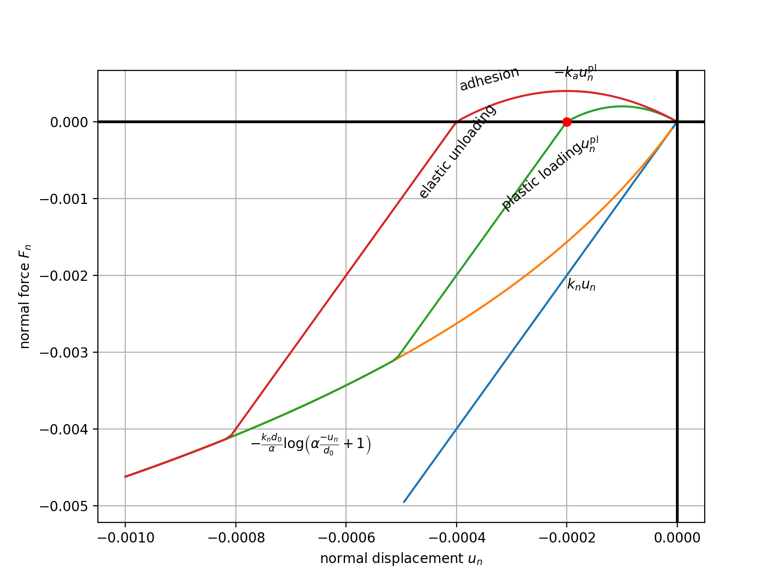
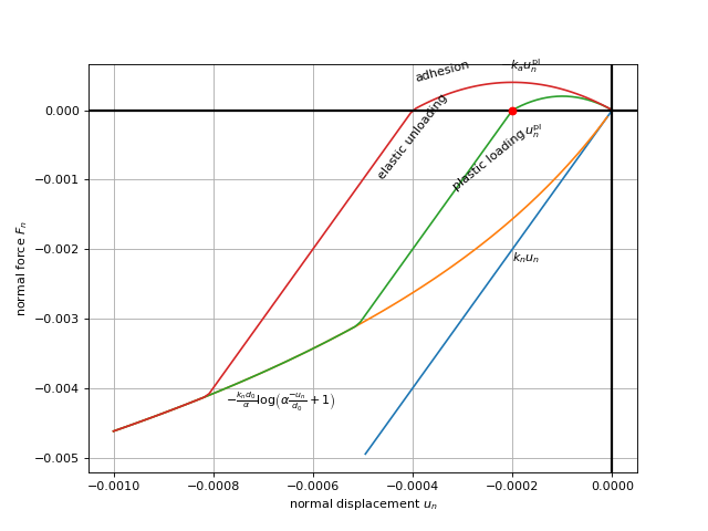
This plot shows the deformation-force diagram with two loading-unloading cycles, showing how plastic deformation and adhesion grow.

(Source code, png, hires.png, pdf)

Energy balance

As this model unloads linearly, elastic potential energy is computed as with the linear model, i.e.

\[E_e=\frac{1}{2}\left(\frac{F_n^2}{k_n}+\frac{|\vec{F}_t|^2}{k_t}\right).\]

Normal plastic dissipation, when normal sliding takes place, is computed using backwards trapezoid integration; the previous yield force is

\begin{align*} \Delta u_n^{\mathrm{pl}}&=\prev{{u_n^{\mathrm{pl}}}}-\curr{{u_n^{\mathrm{pl}}}} \\ \prev{{F_n^y}}&\approx \curr{{F_n^y}} + \frac{\partial F_n^y}{\partial u_n}(\curr{u_n})\Delta u_n^{\mathrm{pl}} \end{align*}

and the normal plastic dissipation

\[\Delta E_{pn}=\frac{1}{2}\left|\prev{{F_n^y}}+\curr{{F_n^y}}\right| \left|\Delta u_n^{\mathrm{pl}}\right|.\]

Tangential plastic dissipation \(\Delta E_{pt}\) is computed the same as for the Linear (Cundall) contact model.

Note

Besides the global energy tracker, the contact law stores the dissipated energy also in PelletMatState, if contacting particles define it. Each particle receives the increment of \(\Delta E_{pn}/2\) (normPlast) and \(\Delta E_{pt}/2\) (shearPlast) . This allows to localize and visualize energy dissipation with the granularity of a single particle – by choosing the appropriate scalar with woo.gl.Gl1_DemField.matStateIx.

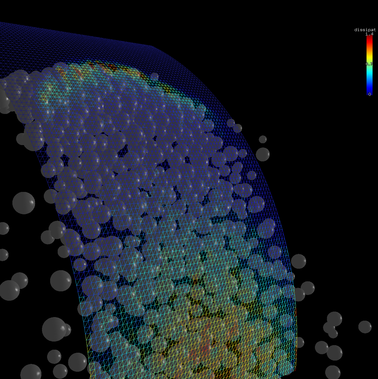
Fig. 14 Spatial distribution of plastic dissipation in the simulation of particle stream impacting a shield.

Confinement

History-independent adhesion can be added by fake confinement \(\sigma_c\) (confSigma) of which negative values lead to constant adhesion.

If \(\sigma_c\) (confSigma) is non-zero, \(F_n\) is updated as

\[F_n \leftarrow F_n-A\sigma_c\]

where \(A\) is the contact area.

To account for the effect of \(\sigma_c\) depending on particle size, \(r_{\mathrm{ref}}\) and \(\beta_c\) (confRefRad and confExp) can be specified, in which case \(F_n\) is updated as

\[F_n \leftarrow F_n-A\sigma_c\underbrace{\left(\frac{A}{\pi r_{\mathrm{ref}}^2}\right)^{\beta_c}}_{\dagger};\]

this leads to the confining stress being scaled by \(\dagger\) – increased/decreased for bigger/smaller particles with \(\beta_c>0\), or vice versa, decreased/increased for bigger/smaller particles with \(\beta_c<0\).

Thinning

Larger-scale deformation of spherical pellets is modeled using an ad-hoc algorithm for reducing particle radius during plastic deformation along with rolling (mass and inertia are not changed, as if the density were accordingly increased). When the contact is undergoing plastic deformation (i.e. \(F_n^t<F_n^y\); notice that \(F_n^y<0\) and \(F_n^t<0\) in compression), then the particle radius is updated.

This process is controlled by three parameters:

1. \(\theta_t\) (thinRate) controlling the amount of radius decrease per unit normal plastic deformation (\(\Delta u_N^{\mathrm{pl}}\)) and unit rolling angle (\(\omega_r\Delta t\), where \(\omega_r\) is the tangential part (\(y\) and \(z\)) of relative angular velocity \(\vec{\omega}_r\)); the unit of \(\theta_t\) is therefore \(\mathrm{1/rad}\) (i.e. dimensionless).

2. \(r_{\min}^{\mathrm{rel}}\) (thinRelRMin), dimensionless, relative minimum particle radius (the original paticle radius is noted \(r_0\)).

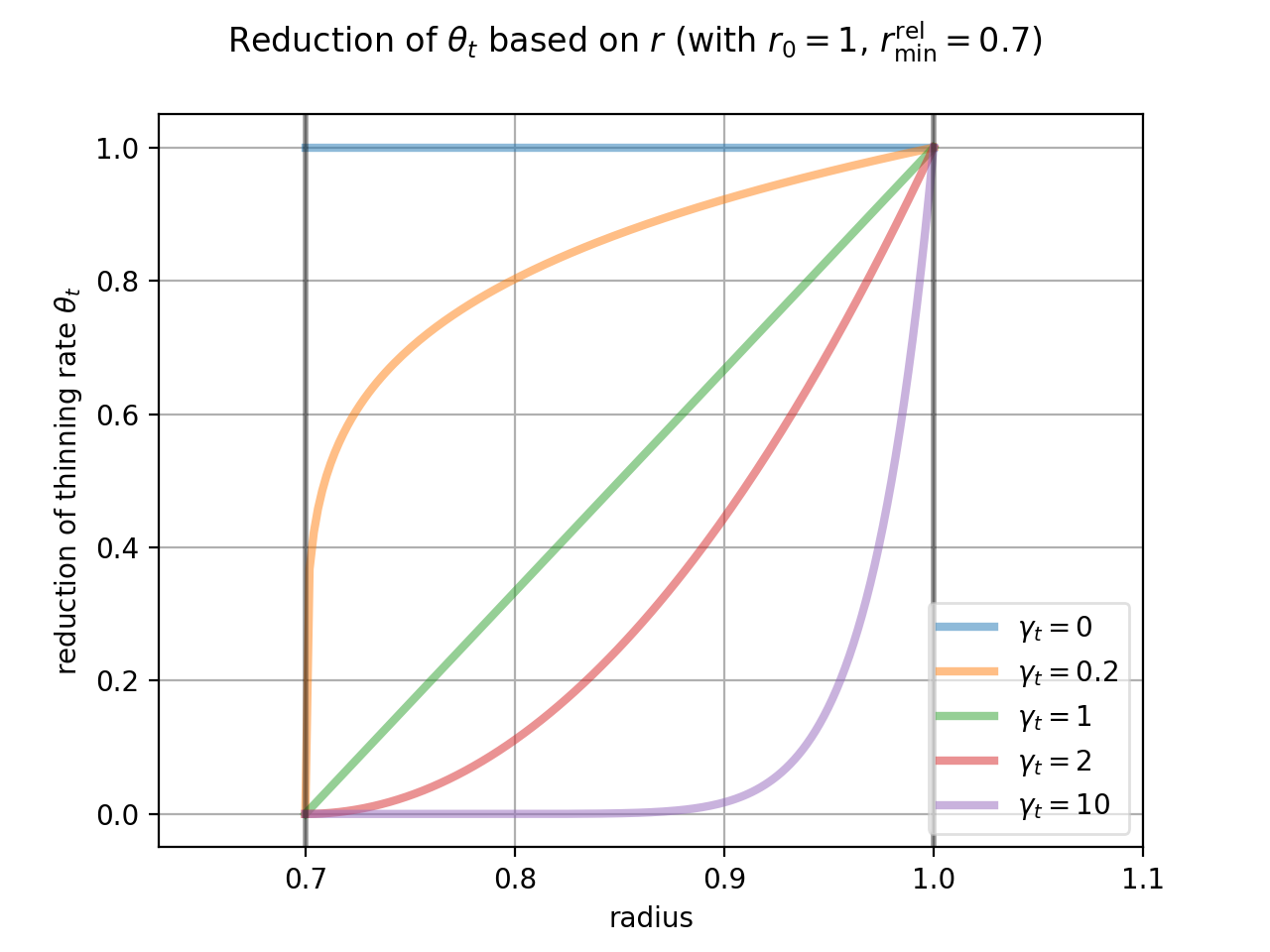
3. \(\gamma_t\) (thinExp), exponent for decreasing the thinning rate as the minimum radius is being approached. The valid range is \(\gamma_t\in\langle 0,\infty)\), otherwise, the reduction is not done (equivalent to \(\gamma_t=0\)). Larger values of \(\gamma_t\) make approaching the radius floor \(r_{\min}^{\mathrm{rel}}\) harder.

(Source code, png, hires.png, pdf)

When thinning is active, the radius is updated as follows:

\begin{align} r_{\min} &= r_{\min}^{\mathrm{rel}} r_0, \tag{*} \\ \Delta u_N^{\mathrm{pl}}&=\curr{(u_N^{\mathrm{pl}})}-\prev{(u_N^{\mathrm{pl}})}, \\ (\Delta r)_0 &=\theta_t \Delta u_N^{\mathrm{pl}} \omega_r \Delta t, \tag{**} \\ \Delta r&=\begin{cases}(\Delta_r)_0 & \gamma_t<0 \\ (\Delta_r)_0\left(\frac{r-r_{\min}}{r_0-r_{\min}}\right)^{\gamma_t} & \mbox{otherwise} \end{cases}, \\ r & \rightarrow \min(r-\Delta r,r_{\min}). \end{align}

Note

Unlike \(u_n^{\mathrm{pl}}\) which is stored per-contact (uNPl) and is zero-initialized for every new contact, the change of radius is permanent. It is possible to recover the original radius in woo.dem.BoxDeleter by setting the recoverRadius flag, which re-computes the radius from mass and density.

Radius-dependence

The \(r_{\min}^{\mathrm{rel}}\) and \(\theta_t\) in the previous can be made effectively size-dependent by setting the \(r_{\rm thinRefRad}\) (thinRefRad) to a positive value. In that case, two additional exponents thinMinExp and thinRateExp are used to multiply the equations \((*)\) and \((**)\) by exponential scaling factors. Note that the dependency is on the original radius \(r_0\), not the current radius \(r\):

\begin{align*} r_{\min} &= \underbrace{\left(\frac{r_0}{r_{\rm thinRefRad}}\right)^{\rm thinMinExp} r_{\min}^{\mathrm{rel}} } r_0, \tag{*} \\ (\Delta r)_0 &=\underbrace{\left(\frac{r_0}{r_{\rm thinRefRad}}\right)^{\rm thinRateExp} \theta_t} \Delta u_N^{\mathrm{pl}} \omega_r \Delta t. \tag{**} \\ \end{align*}

Tip

Report issues or inclarities to github.