Linear (Cundall) contact model

Linear contact model is widely used throughout the DEM field and was first published in [CS79]. Normal force is linear function of normal displacement (=overlap); shear force increases linearly with relative shear displacement, but is limited by Coulomb linear friciton. This model is implemented in woo.dem.Law2_L6Geom_FrictPhys_IdealElPl.

Stiffness

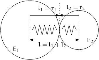
Fig. 13 Series of 2 springs representing normal stiffness of contact between 2 spheres.

Normal stiffness is related to Young modulus of both particles’ materials. For clarity, we define contact area of a fictious “connector” between spheres of total length \(l=l_1+l_2\). These effective lengths are equal to radii for spheres (but have other values for e.g. walls or facets – see below), minus the initial overlap. The contact area is

(2)\[A=\pi\min(l_1,l_2)^2\]

where \(l_i\) is (equivalent – for non-spheres) radius the respective particle. The connector is therefore an imaginary cylinder with radius of the lesser sphere, spanning between their centers. Its stiffness is then

(3)\[k_n=\left(\frac{l_1}{E_1 A}+\frac{l_2}{E_2 A}\right)^{-1}.\]

Tangent (shear) stiffness \(k_t\) is a fraction (ktDivKn) of \(k_n\),

(4)\[k_t=\left(\frac{k_t}{k_n}\right)k_n,\]

where the ratio is averaged between both materials in contact.

Friction angle on the contact is computed from contacting materials as

\[\tan\phi=\min\left[(\tan\phi)_1,(\tan\phi)_2\right],\]

(unless specified otherwise) of which consequence is that material without friction will not have frictional contacts, regardless of friction of the other material.

Note

It is a simplification to derive friction parameters from material properties – the interface of each couple of materials might have different parameters, though this simplification is mostly sufficient in the practice. If you need to define different parameters for every combination of material instances, there is the woo.core.MatchMaker infrastructure.

Non-spherical particles

The formulas for spheres above suppose that there is particle radius (radius) which defines mechanically active length (between contact point and centroid) where the material deforms (\(l_1\), \(l_2\)). This is generalized for contact of non-spherical particles, but there are often choices which have to balance computing performance, (somewhat subjective) intuition and (perceived) physical correctness.

The rules for determining \(l_i\) are the following:

1. Round particles contacting between themselves (including Facet with non-zero halfThick use their natural radii: Sphere.radius, Facet.halfThick, Capsule.radius, InfCylidner.radius, computed centroid – contact point distance for Ellipsoid).

2. Flat particles (Wall or Facet with zero halfThick) use the other’s particle radius – this results in the same influence on contact parameters from both particles, which accounts for local (not simulated) deformation of those flat particles.

As a special case, Facet + Sphere set \(l_1\) equal to max(halfThick, radius) and \(l_2\) to radius. The max is to account for facets with both zero and non-zero halfThick.

3. Contact of 2 flat particles is undefined.

These rules are implemented in Cp2_ functors for respective shape combinations, and are passed as parameters to Cg2_Any_Any_L6Geom__Base::handleSpheresLikeContact and to Cp2_FrictMat_FrictPhys::updateFrictPhys in turn. Refer to their source code for details.

Examples

1. Capsule in contact with Sphere, with

   \begin{align*} r_1&=.2\,\mathrm{m}, & r_2&=.1\,\mathrm{m}, \\ u_N&=.001\,\mathrm{m}, \\ E_1&=10\,\mathrm{MPa}, & E_2&=30\,\mathrm{MPa}, \\ l_1&=r_1-\frac{u_N}{2}, & l_2&=\frac{u_N}{2}, \\ A&=\pi\min(l_1,l_2)^2, \\ \end{align*}

   lead to equivalent modulus and stiffness:

   \begin{align*} \frac{l}{E'}&=\frac{l_1+l_2}{E'}=\frac{l_1}{E_1}+\frac{l_2}{E_2}, \\ k_n=\frac{E'A}{l}&=A\left(\frac{l_1}{E_1}+\frac{l_2}{E_2}\right)^{-1} \end{align*}

   Woo[1]: r1,r2=.2,.1; uN=-.001; E1,E2=10e6,30e6
   
   Woo[2]: S1=Scene(fields=[DemField(par=[Capsule.make((0,0,0),radius=r1,shaft=.1,mat=FrictMat(young=E1)),Sphere.make((0,0,r1+r2+uN),radius=r2,mat=FrictMat(young=E2))])],engines=DemField.minimalEngines())
   
   Woo[3]: S1.one(); c=S1.dem.con[0] # one step to create contact
   
   Woo[4]: c.geom.lens, c.geom.contA, c.phys.kn
   Out[4]: (Vector2(0.1,0.2), 0.031415926535897934, 1346396.8515384828)
   
   # recompute by hand to check:
   Woo[5]: l1,l2=r1+uN/2.,r2+uN/2.; A=pi*min(l1,l2)**2
   
   # l1,l2 swapped above since the functor Cg2_Sphere_Capsule_L6Geom reorders the contact
   Woo[6]: (l2,l1), A, A*(l1/E1+l2/E2)**-1
   Out[6]: ((0.0995, 0.1995), 0.031102552668702352, 1336785.9313195853)
   

2. thin Facet (with \(h=0\) as halfThick) in contact with Sphere, with

   \begin{align*} h&=0\,\mathrm{m}, & r&=.1\,\mathrm{m}, \\ u_N&=.001\,\mathrm{m}, \\ E_1&=10\,\mathrm{MPa}, & E_2&=30\,\mathrm{MPa}, \\ l_1&=\max(h,r)-\frac{u_N}{2}, & l_2&=r-\frac{u_N}{2}, \\ A&=\pi\min(l_1,l_2)^2 \end{align*}

   Woo[7]: h,r=0,.1; uN=-.001; E1,E2=10e6,30e6;
   
   Woo[8]: S2=Scene(fields=[DemField(par=[Facet.make([(0,0,0),(1,0,0),(0,1,0)],halfThick=h,mat=FrictMat(young=E1)),Sphere.make((.2,.2,h+r+uN),radius=r,mat=FrictMat(young=E2))])],engines=DemField.minimalEngines())
   
   Woo[9]: S2.one(); c=S2.dem.con[0] # one step to create contact
   
   Woo[10]: c.geom.lens, c.geom.contA, c.phys.kn
   Out[10]: (Vector2(0.1,0.1), 0.031415926535897934, 2356194.4901923453)
   
   # hand-computation
   Woo[11]: l1,l2=max(h,r)+uN/2.,r+uN/2.; A=pi*min(l1,l2)**2
   
   Woo[12]: (l1,l2), A, A*(l1/E1+l2/E2)**-1
   Out[12]: ((0.0995, 0.0995), 0.031102552668702352, 2344413.5177413835)
   

   Warning

   The above does not match?! Should be tracked down.

Contact respose

Normal response is computed from the normal displacement (or overlap) as

\[F_n=u_n k_n\]

and the contact is (optionally) broken when \(u_n>0\).

Trial tangential force is computed from tangential relative velocity \(\dot u\) incrementally and finally (optionally) reduced by the coulomb Criterion. Tangential force is a 2-vector along contact-local \(y\) and \(z\) axes.

\begin{align*} \Delta \vec{F}_t&=(\pprev{\vec{\dot u}})_t\Dt k_t, \\ \vec{F}_t^T&=\curr{\vec{F}_t}+\Delta \vec{F}_t, \end{align*}

and total tangential force is reduced by the Coulomb criterion:

\[\begin{split}\next{\vec{F}_t}=\begin{cases} \curr{\vec{F}_t}+\Delta \vec{F}_t & \text{if } |\curr{\vec{F}_t}+\Delta \vec{F}_t|<F_n\tan\phi, \\ F_n\tan\phi\frac{\curr{\vec{F}_t}+\Delta \vec{F}_t}{|\cdot|} & \text{otherwise}. \end{cases}\end{split}\]

Energy balance

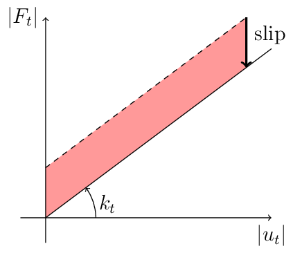
Elastic potential stored in a contact is the contact is the triangular area below the displacement-force diagram, in both normal and tangent sense,

\[\frac{1}{2}\left(\frac{F_n^2}{k_n}+\frac{|\vec{F}_t|^2}{k_t}\right).\]

Plastically dissipated energy is the elastic energy removed by the tangent slip. Noting \(f_y=F_n\tan\phi\) (yield force magnitude), and norm of the trial tangent force \(f_t=|\curr{\vec{F}_t}+\Delta\vec{F}_t|\), this energy can be seen as the red area (parallelogram) in the displacement-force diagram

leading to

\[\Delta E_{pt}=\frac{f_t-f_y}{k_t}f_y.\]

Todo

The code has a different formulation: one contribution of \(\frac{1}{2}\frac{f_t-f_y}{k_t}(f_t-f_y)\) and another of \(f_y\frac{f_t-f_y}{k_t}\), giving together

\[\Delta E_{pt}=\left(\frac{f_t-f_y}{2}+f_y\right)\frac{f_t-f_y}{k_t}.\]

The difference of elastic potentials leads to yet another formulation:

\[\Delta E_{pt}=\frac{1}{2}\frac{f_t^2}{k_t}-\frac{1}{2}\frac{f_y^2}{k_t}=\frac{f_t^2-f_y^2}{2k_t}.\]

Decide analytically on which of those is the best approximation and use it both in the code and in the docs.

Purely elastic model 6-DoF model

This model is useful for testing purposes. It has elastic response along all 6 DoFs: normal displacement, 2 shear displacements, twisting and 2 bending rotations. There is no non-linearity (like plastic beahvior). The model is implemented in woo.dem.Law2_L6Geom_FrictPhys_LinEl6. For simplicity, it uses woo.dem.FrictPhys (ignoring tanPhi) to compute elastic parameters, plus an additional attribute charLen to compute rotational stiffnesses. Thus the stiffnesses are as follows:

• normal and tangential stiffnesses kn, kt are computed as above in eqs. (3), (4). Their dimension is N/m² as usual.

• bending stiffnesses \(k_w\) (twist) and \(k_b\) (bending) have the dimension N/m and are computed using the factor \(l\) (charLen), which ensures dimensional consistency, as

\begin{align*} k_w&=l k_n, & k_b&=l k_s, \end{align*}

which means that \(k_t/k_n=k_b/k_w\); this should be acceptable since the model is used for testing only.

Contact forces are computed strictly elastically as

\begin{align*} F_n&=k_n u_n, & \vec{F}_t&=k_t \vec{u}_t, \\ T_n&=k_w \phi_n, & \vec{T}_b&=k_b \vec{\phi}_t. \end{align*}

Stored elastic energy is computed as

\[E_e=\frac{1}{2}\left(\frac{F_n^2}{k_n}+\frac{|\vec{F}_t|^2}{k_t}+\frac{T_n}{k_w}+\frac{|\vec{T}_b|^2}{k_b}\right)\]

with careful handling of zero stiffnesses so that the expression is numerically sound.

Tip

Report issues or inclarities to github.