Concrete contact model

Note

This model was originally published in in the thesis [Smi10] under the name Concrete Particle Model (CPM) and ported from Yade to Woo by the author. This page was converted from the thesis source.

Contact law is formulated on the level of individual contacts between 2 particles. However, since desired results are macroscopic and not observed until larger simulations are performed, motivations for introducing various contact-level features of the model might not be obvious until after reading Parameter calibration.

Prior discrete concrete models

Before describing the CPM model, we would like to give a brief overview of some of the main particle-based, DEM and non-DEM, concrete models.

Lattice models

[Ver97] (pg. 14-16) gives an overview of older lattice models used for concrete. Later lattice models of concrete aim usually at meso-scale modeling, where aggregates and mortar are distinguished by differing beam parameters. Beam configuration can be regular (leading to failure anisotropy), random [LvM03], or generated to match observed statistical distribution [LSM04].

[LvM03] uses brittle beam behavior, simply removing broken beams from simulation; [LSM04] uses tensile softening to avoid dependence of global softening (which is observed even with brittle behavior of beams) on beam size. Neither of these models focuses on capturing compression behavior.

[CBavzantC03] presents a rather sophisticated model, in which properties of lattice beams are computed from the geometry of Voronoï cells of each node. Granulometry is supposed to have substantial influence on confinement behavior; as it is not fully considered by the model, the beam-transversal stress history influences shear rigidity instead. Compression behavior is captured fairly well.

Rigid body – spring models

This family of models is, to our knowledge, used infrequently for concrete. [NSUK02] presents a mesoscopic (distinguishing aggregates and mortar) model, though only formulated in 2D.

Discrete element models

Such of concrete are rather rare. Most activity (judging by publications) comes from teams formed around Frédéric V. Donzé. His work (using SDEC software, see https://yade-dem.org/wiki/Yade_history for details)) first targeted at 2D DEM [CMDonze00]. Later, exploiting the dynamic nature of DEM led to fast concrete dynamics in 3D [Hen03] [HDD04] and impact simulation [SDonzeD08]. In order to reduce computational costs, elastic FEM for the non-damaged subdomain is used, with some tricks to avoid spurious dynamic effects on the DEM/FEM boundary [RFMD09].

With both lattice and DEM models, arriving at reasonable compression behavior is non-trivial; it seems to stem from the fact that 1D elements (beams in lattice, bonds in DEM) have no notion of an overall stress state at their vicinity, but only insofar as it is manifested in the direction of the respective element. [CBavzantC03] works around this by explicitly introducing the influence of transversal stress. [Hen03] (sect. 5.3), on the other hand, blocks rotations of spherical elements to achieve a higher and more realistic $f_c/f_t$ ratio, but it is questionable whether there is physically sound reason for such an adjustment.

Model description

Cohesive and non-cohesive contacts

We use the word contact to denote both cohesive (material bond) and non-cohesive (contact two spheres meeting during their motion) contacts, as they are governed by the same equations. The non-cohesive contact only differs by that it is considered as fully damaged from the very start, by setting the damage variable $\omega=1$; since damage effectively prevent tensile forces in the contact, the result is that the two spheres interact only while in tension (geometrically overlapping) and disappears when they geometrically separate. On the other hand, cohesive contact, which is always created at the beginning of the simulation, is created in virgin, undamaged state.

Contact parameters

As already explained above, most parameters of a contact are computed as averages of particle material properties. That is also true for the CPM model, with the respective material and Cp2 functor classes.

Those computed as averages (from values that are typically identical, since particles share the same material) are $c_{T0}$, $\eps_0$, $\eps_s$, $k_N$ (from particles’ moduli $E$), $\tau_d$, $M_d$, $\tau_{pl}$, $M_{pl}$, $\sigma_0$, $\phi$. (The meaning of symbols used here is explained in the following text.)

On the other hand, shear modulus $k_T$ is computed from $k_N$ using the ratio in ktDivKn. $\eps_f$ is computed from $\eps_0$ by multiplying it by dimensionless relDuctility, which is $\eps_f/\eps_0$.

Finally, some parameters are set in the woo.dem.Law2_L6Geom_ConcretePhys law functor, hence the same for all interactions. Those are $Y_0$ and $\tilde K_s$.

Density of the particle material is set to $\rho=4800\,{\rm kgm^{-3}}$ (by default), as we have to compensate for porosity of the packing, which a little above 50% for spheres of the same radius and we take continuum concrete density roughly $2400\,{\rm kgm^{-3}}$.

Normal stresses

The normal stress-strain law is formulated within the framework of damage mechanics:

(15) $$\sigma_N =[1-\omega H(\eps_N)] k_N\eps_N.$$

Here, $k_N$ is the normal modulus (model parameter, [Pa]), and $\omega\in\langle0,1\rangle$ is the damage variable. The Heaviside function $H(\eps_N)$ deactivates damage influence in compression, which physically corresponds to crack closure.

The damage variable $\omega$ is evaluated using the damage evolution function $g$ (figure):

$$\begin{align} \omega=g(\kappa)&=1-\frac{\eps_f}{\kappa}\exp\left(-\frac{\kappa-\eps_0}{\eps_f}\right)\\ \kappa&=\max \tilde\eps\\ \tilde\eps&=\sqrt{\langle\eps_N\rangle^2+\xi_1^2|\eps_T|^2}, \end{align}$$

where $\tilde\eps$ is the equivalent strain responsible for damage ($\langle\eps_N \rangle$ signifies the positive part of $\eps_N$) and $\xi_1$ is a dimensionless coefficient weighting the contribution of the shear strain $\eps_T$ to damage. However, comparative studies indicate that the optimal value is $\xi_1\equiv 0$, hence equation (16) simplifies to $\tilde\eps=\langle\eps_N\rangle$. $\kappa$ is the maximum equivalent strain over the whole history of the contact.

Fig. 15 Damage $\omega$ evolution function $\omega=g(\kappa_D)$, where $\kappa_D=\max \eps_N$ (using $\eps_0=0.0001$, $\eps_f=30\eps_0$).

Parameter $\eps_0$ is the limit elastic strain, and the product $K_T\eps_0$ corresponds to the local tensile strength at the level of one contact (in general different from the macroscopic tensile strength). Parameter $\eps_f$ is related to the slope of the softening part of the normal strain-stress diagram (figure) and must be larger than $\eps_0$.

Fig. 16 Strain-stress diagram in the normal direction.

Compressive plasticity

To better capture confinement effect, we introduce, as an extension to the model, hardening in plasticity in compression. Using material parameter $\eps_s<0$, we define $\sigma_s=k_N\eps_s$. If $\sigma<\sigma_s$, then $\tilde K_s k_N$ is taken for tangent stiffness, $\tilde K_s \in\langle0,1\rangle$ and plastic strain $\eps_N^{\rm pl}$ is incremented accordingly. This introduces 2 new parameters $\eps_s$ (stress at which the hardening branch begins) and $\tilde K_s$ (relative modulus of the hardening branch) that must be calibrated (see Parameter calibration) and one internal variable $\eps_N^{\rm pl}$.

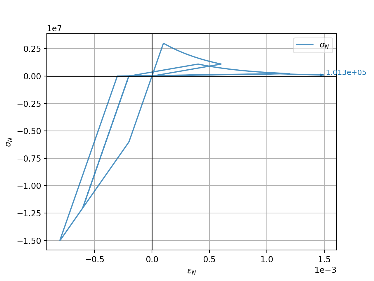
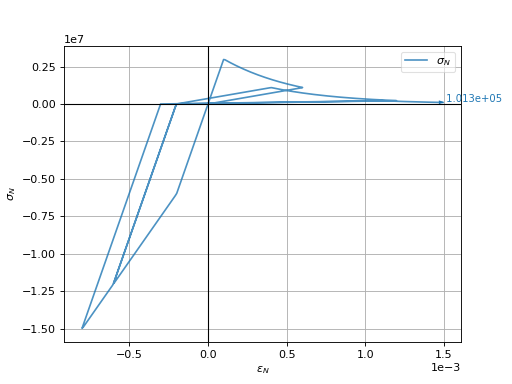
Extended strain-stress diagram for multiple loading cycles is shown in this figure. Note that this feature is activated only in compression, whereas damage is activated only in tension. Therefore, there is no need to specially consider interaction between both.

This following is the strain-stress diagram in normal direction, loaded cyclically in tension and compression; it shows several features of the model: (1) damage in tension, but not damage in compression (governed by the $\omega$ internal variable) (2) plasticity in compression, starting at strain $\eps_s$; reduced (hardening) modulus is $\tilde K_s k_N$:

(Source code, png, hires.png, pdf)

Visco-damage

In order to model time-dependent phenomena, viscosity is introduced in tension by adding viscous overstress $\sigma_{Nv}$ to (15). As we suppose it to be related to a limited rate of crack propagation, it cannot depend on total strain rate; rather, we split total strain into the elastic strain $\eps_e$ and the damage part $\eps_d$. Since $\eps_e=\sigma_N/k_N$, we have

(17) $$\eps_d=\eps_N-\frac{\sigma_N}{k_N}.$$

We then postulate the overstress in the form

(18) $$\sigma_{Nv}(\dot\eps_d)=k_N\eps_0\langle\tau_d\dot\eps_{Nd}\rangle^{M_d},$$

where $k_N\eps_0$ is rate-independent tensile strength (introduced for the sake of dimensionality), $\tau_d$ is characteristic time for visco-damage and $M_d$ is a dimensionless exponent. The $\langle\dots\rangle$ operator denotes positive part; therefore, for $\dot\eps_{Nd}\leq0$, viscous overstress vanishes. 2 new parameters $\tau_d$ and $M_d$ were introduced.

The normal stress equation then reads

(19) $$\sigma_N=\left[1-\omega H(\eps_N)\right]k_N\eps_N+\sigma_{Nv}(\dot \eps_{Nd}).$$

In a finite step computation, we can evaluate the damage variable $\omega$ in a rate-independent manner first; then, we compute the increment of $\eps_d$ satisfying equations (17)–(19). As usual, we use $\curr{\bullet}$, $\next{\bullet}$ to denote value of $\bullet$ at $t$, $t+\Dt$ (at the beginning and at the end of the current timestep) respectively. We approximate the damage strain rate by the difference formula

$$\dot\eps_d=\frac{\next{\eps}_d-\curr{\eps}_d}{\Delta t}=\frac{\Delta\eps_d}{\Delta t}$$

and substitute (18) and (19) into (17) obtaining

$$\curr{\eps}_d+\Delta\eps_d=\next{\eps}_N-(1-\omega)\next{\eps}_N-\frac{k_N\eps0}{k_N}\left\langle\frac{\tau_d\Delta\eps_d}{\Delta t}\right\rangle^{M_d},$$

which can be written as

(20) $$\Delta\eps_d+\eps_0\left\langle\frac{\tau_d\Delta\eps_d}{\Delta t}\right\rangle^{M_d}=\omega\next{\eps}_N-\curr{\eps}_d$$

During unloading, i.e. $\Delta\eps_d\leq0$, the power term vanishes, leading to

$$\Delta\eps_d=\omega\next{\eps}_N-\curr{\eps}_d,$$

applicable if $\omega\next{\eps}_N\leq\curr{\eps}_d$.

In the contrary case, (20) must be solved, but $\langle\cdots\rangle$ can be replaced by $(\cdots)$ since the term is now known to be positive. We divide (20) by its right-hand side and apply logarithm. We transform the unknown $\Delta\eps_d$ into a new unknown

(21) $$\beta=\ln\frac{\Delta\eps_d}{\omega\next{\eps}_N-\curr{\eps}_d},$$

obtaining the equation

(22) $$\ln\left({\rm e}^\beta+c{\rm e}^{M_d\beta}\right)=0,$$

with

$$c=(1-\omega)\eps_0\left(\omega\next{\eps}_N-\curr{\eps}_d\right)^{M_d-1}\left(\frac{\tau_d}{\Delta t}\right)^{M_d}.$$

For positive $c$ and $M_d$, the term $\ln({\rm e}^\beta+c{\rm e}^{M_d\beta})$ from (22)) is convex, increasing and positive at $\beta=0$. As a consequence, the Newton method with starting point at $\beta=0$ always converges monotonically to a unique negative solution of $\beta$. (Using pre-determined maximum number of steps and given absolute tolerance $\delta$, we start with $\beta=0$. Then at each step, we compute $a=c\exp(N\beta)+\exp(N)$ and $f=\log(a)$. If $|f|<\delta$, then $\beta$ is the desired solution. Otherwise, we update $\beta\leftarrow\beta-f/((cN\exp{N\beta}+\exp{\beta})/a)$ and continue with the next step.)

From the solution $\beta$, we compute

$$\Delta\eps_d=\left(\omega\next{\eps}_N-\curr{\eps}_d\right){\rm e}^\beta.$$

Finally, the term $\sigma_{Nd}(\dot\eps_d)=\sigma_{Nd}\left(\frac{\Delta\eps_d}{\Delta t}\right)$ in (18) can be evaluated and plugged into (19).

The effect of viscosity on damage for one contact is shown in the following figure; calibration of the new parameters $\tau_d$ and $M_d$ is described in Parameter calibration.

Fig. 17 Strain-stress curve in tension with different rates of loading; the parameters used here are $\tau_d=1\,{\rm s}$ and $M_d=0.1$.

Isotropic confinement

During calibration, we faced the necessity to simulate confined compression setups. Applying boundary confinement on a specimen composed of many particles is not straightforward, since thera are necessary strong local effects. We then found a way to introduce isotropic confinement at contact level, by pre-adjusting $\eps_N$ and post-adjusting $\sigma_N$; the supposition is that the confinement value $\sigma_0$ is negative and does not lead to immediate damage to contacts.

Given a prescribed confinement value $\sigma_0$, we adjust $\eps_N$ value before computing normal and shear stresses:

$$\begin{split}\eps_N'=\eps_N+\begin{cases} \sigma_0/k_N & \hbox{if $\sigma_0>k_N\eps_s$,} \\ \eps_s+\frac{\sigma_0-k_N\eps_s}{k_N\tilde K_s} & \hbox{otherwise,} \\ \end{cases}\end{split}$$

where the second case takes in account compressive plasticity. The constitutive law then uses the adjusted value $\eps_N'$. At the end, computed normal stress is adjusted back to

$$\sigma_N'=\sigma_N-\sigma_0$$

before being applied on particle in contact.

Shear stresses

For the shear stress we use plastic constitutive law

$$\vec{\sigma}_T=k_T(\vec{\eps}_T-\vec{\eps}_{Tp})$$

where $\eps_{Tp}$ is the plastic strain on the contact and $k_T$ is shear contact modulus computed from $k_N$ as the ratio $k_T/k_N$ is fixed (usually 0.2, see the Parameter calibration).

XXX In the DEM formulation (large strains), however, $\vec{\eps}_{Tp}$ is not stored and mapped contact points on element surfaces are moved instead as explained above, sect.~ref{sect-formulation-total-shear}.

The shear stress is limited by the yield function (figure)

(23) $$\begin{align}\begin{aligned}f(\sigma_N,\vec{\sigma}_T)&=|\vec{\sigma}_T|-r_{pl}=|\vec{\sigma}_T-(c_T-\sigma_N\tan\phi),\\c_T&=c_{T0}(1-\omega)\end{aligned}\end{align}$$

where material parameters $c_{T0}$ and $\phi$ are initial cohesion and internal friction angle, respectively. The initial cohesion $c_{T0}$ is reduced to the current cohesion $c_T$ using damage state variable $\omega$. Note that we split the plasticity function in a part that depends on $\vec{\sigma}_T$ and another part which depends on already known values of $\omega$ and $\sigma_N$; the latter is denoted $r_{pl}$, radius of the plasticity surface in given $\sigma_N$ plane.

The plastic flow rule

$$\vec{\dot\eps}_{Tp}=\dot\lambda\frac{\vec{\sigma}_T}{|\vec{\sigma}_T|},$$

$\lambda$ being plastic multiplier, is associated in the plane of shear stresses but not with respect to the normal stress (figure). The advantage of using a non-associated flow rule is computational. At every step, $\sigma_N$ can be evaluated directly, followed by a direct evaluation of $\vec{\sigma}_T$; stress return in shear stress plane reduces to simple radial return and does not require any iterations as $f(\sigma_N,\vec{\sigma}_T)=0$ is satisfied immediately.

In the implementation, numerical evaluation starts from current value of $\vec{\eps}_T$. Trial stress $\vec{\sigma}_T^t=\vec{\eps}_T k_T$ is computed and compared with current plasticity surface radius $r_{pl}$ from (23). If $|\vec{\sigma}_T^t|>r_{pl}$, the radial stress return is performed; since we do not store $\vec{\eps}_{Tp}$, $\vec{\eps}_T$ is updated as well in such case:

$$\begin{align} \vec{\sigma}_T&=r_{pl} \normalized{\vec{\sigma_T}} \\ \vec{\eps}_T'&=\normalized{\vec{\eps}_T}\frac{|\vec{\sigma}_T|}{|\vec{\sigma}_T^t|} \end{align}$$

If $|\vec{\sigma}_T^t|\leq r_{pl}$, there is no plastic slip and we simply assign $\vec{\sigma}_T=\vec{\sigma}_T^t$ without $\vec{\eps}_T$ update.

Fig. 18 Linear yield surface and plastic flow rule.

Confinement extension

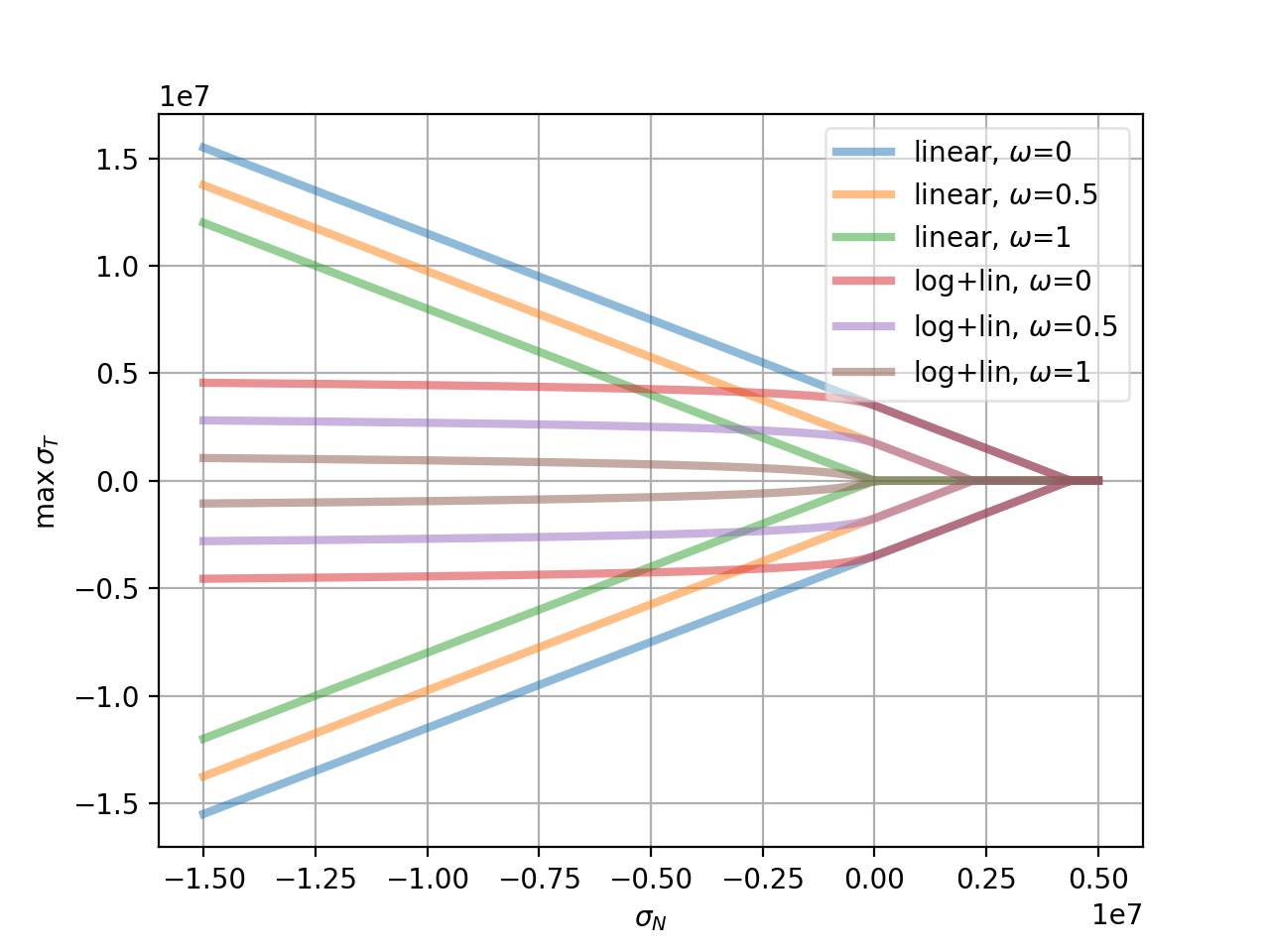
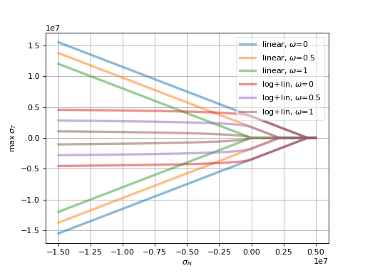
As in the case of normal stress, we introduce an extension to better capture confinement effect and to prevent shear locking under extreme compression: instead of using linear plastic surface we replace it by logarithmic surface in the compression part, which has $C_1$ continuity with the linear surface in tension; the continuity condition avoids pathologic behavior around the switch point and also reduces number of new parameters. Instead of (23), we use

$$\begin{split}f(\sigma_N,\sigma_T)= \begin{cases} |\sigma_T|-(c_{T0}(1-\omega)-\sigma_N\tan\phi) & \hbox{if } \sigma_N\geq0 \\ |\sigma_T|-c_{T0}\left[(1-\omega)+Y_0\tan\phi\log\left(\frac{-\sigma_N}{c_{T0} Y_0}+1\right)\right] & \hbox{if } \sigma_N<0, \end{cases}\end{split}$$

which introduces a new dimensionless parameter $Y_0$ determining how fast the logarithm deviates from the original, linear form. The function is shown, and compared with the linear function, for both virgin and damaged material, in this figure:

(Source code, png, hires.png, pdf)

Visco-plasticity

Viscosity in shear uses similar ideas as visco-damage from sect.~ref{sect-cpm-visco-damage}; the value of $r_t$ in (23) is augmented depending on rate of plastic flow following the equation

$$r_{pl}'=r_{pl}+c_{T0}\left(\tau_{pl}\vec{\dot\eps}_{Tp}\right)^{M_{pl}}=r_{pl}+c_{T0}\left(\tau_{pl}\frac{\Delta\vec{\eps}_{Tp}}{\Dt}\right)^{M_{pl}}$$

where $\tau_{pl}$ is characteristic time for visco-plasticity, $M_{pl}$ is a dimensionless exponent (both to be calibrated. $c_{T0}$ is undamaged cohesion introduced for the sake of dimensionality.

Similar solution strategy as for visco-damage is used, with different substitutions

$$\begin{align} \beta&=\ln\left(\frac{|\vec{\sigma}_T^t|-r_{pl}'}{|\vec{\sigma}_T^t|-r_{pl}}\right), \\ c&=c_{T0}\left(|\vec{\sigma}_T^t|-r_{pl}\right)^{M_{pl}-1}\left(\frac{\tau_{pl}}{k_T \Dt}\right)^{M_{pl}}. \end{align}$$

The equation to solve is then formally the same as (22)

$$\ln\left({\rm e}^\beta+c{\rm e}^{M_{pl}\beta}\right)=0.$$

After finding $\beta$ using the Newton-Raphson method, trial stress $\vec{\sigma}_T^t$ is scaled by the factor

$$\frac{r'_{pl}}{|\vec{\sigma}_T^t|}=1-e^\beta\left(1-\frac{r_{pl}}{|\vec{\sigma}_T^t|}\right)$$

to obtain the final shear stress value

$$\vec{\sigma}_T=\frac{r'_{pl}}{|\vec{\sigma}_T^t|}\vec{\sigma}_T^t.$$

Applying stresses on particles

Resulting stresses $\sigma_N$ and and $\vec{\sigma}_T$ are computed at the current contact point $\curr{\vec{C}}$. Summary force $\vec{F}_{\Sigma}=A_{eq}(\sigma_N\vec{n}+\vec{\sigma}_T)$ has to be applied to particle’s positions $\curr{\vec{C}}_1$, $\curr{\vec{C}}_2$, exerting force and torque:

$$\begin{align} \vec{F}_1&=\vec{F}_{\Sigma}, & \vec{T}_1&=(\curr{\vec{C}}-\curr{\vec{C}}_1)\times \vec{F}_{\Sigma}, \\ \vec{F}_2&=-\vec{F}_{\Sigma}, & \vec{T}_2&=-(\curr{\vec{C}}-\curr{\vec{C}}_1)\times \vec{F}_{\Sigma}. \end{align}$$

Forces and torques on particles from multiple interactions accumulate during one computation step.

Contact model summary

The computation described above proceeds in the following order:

1. Isotropic confinement $\sigma_0$ is applied if active. This consists in adjusting normal strain to either $\eps_N\leftarrow\eps_N+\sigma_0$ (if $\sigma_0\geq k_N\eps_s$) or $\eps_N\leftarrow\eps_s+(\sigma_0-k_N\eps_s)/(k_N\tilde K_s)$.

2. Normal stress $\sigma_N$. $\tilde\eps=\langle\eps_N\rangle$ is computed, then the history variable is updated $\kappa\leftarrow\max(\kappa,\tilde\eps)$; $\kappa$ is the state variable from which the current damage $\omega=g(k)=1-(\eps_f/\kappa)\exp(-(\kappa-\eps_0)/\eps_f)$ is evaluated; for non-cohesive contacts, however, we set $\omega=1$. For cohesive contacts with damage disabled (ConcretePhys.neverDamage), we set $\omega=0$.

   The state variable $\eps_N^{\rm pl}$ (initially zero) holds the normal plastic strain; we use it to compute the elastic part of the current strain $\eps_N^{\rm el}=\eps_N-\eps_N^{\rm pl}$.

   Normal stress is computed using the equation of damage mechanics $\sigma_N=(1-H(\eps_N^{\rm el})\omega)k_N\eps_N^{\rm el}$.

   Whether compressive hardening is present is determined; $\sigma_{Ns}=k_N(\eps_s+\tilde K_s(\eps_N-\eps_s))$ is pre-evaluated; then if $\eps_N^{\rm el}<\eps_s$ and $\sigma_{Ns}>\sigma_N$, normal stress and normal plastic strains are updated $\eps_N^{\rm pl}\leftarrow \eps_N^{\rm pl}+(\sigma_N-\sigma_{Ns})/k_N$, $\sigma_N\leftarrow\sigma_{Ns}$. If the condition is not satisfied, compressive plasticity has no effect and does not have to be specifically considered.

3. Shear stress $\vec{\sigma}_T$. First, trial value is computed simply from $\vec{\sigma}_T\leftarrow k_T\eps_T$. This value will be compared with the radius of plastic surface $r_{pl}$ for given, already known $\sigma_N$. As there are different plasticity functions for tension and compression, we obtain $r_{pl}=c_{T0}(1-\omega)-\sigma_N\tan\phi$ for $\sigma_N\geq0$; in compression, the logarithmic surface makes the formula more complicated, giving $r_{pl}=c_{T0}\left[(1-\omega)+Y_0\tan\phi(-\sigma_N/(c_{T0}Y_0)+1)\right]$.

   If the trial stress is beyond the admissible range, i.e. $|\vec{\sigma}_T|>r_pl$, plastic flow will take place. Since the total formulation for strain is used, we update the $\vec{\eps}_T$ to have the same direction, but the magnitude of $|\vec{\sigma}_T|/k_T$.

   Without visco-plasticity (the default), a simple update $\vec{\sigma}_T\leftarrow (\sigma_T/|\sigma_T|)r_{pl}$ is performed during the plastic flow. If visco-plasticity is used, we update $\vec{\sigma}_T\leftarrow s\vec{\sigma}_T$, $s$ being a scaling scalar. It is computed as $s=1-e^{\beta}(1-r_{pl}/|\vec{\sigma}_T|)$, where $\beta$ is solved with Newton-Raphson iteration as described above, with the coefficient $c=c_{T0}(\tau_{pl}/(k_T\Dt))^{M_{pl}}(|\vec{\sigma}_T|-r_{pl})^{M_{pl}-1}$ and the exponent $M_{pl}$.

4. Viscous normal overstress $\sigma_{Nv}$ is applied for cohesive contacts only. As explained above, it is effective for non-zero damage rate. When damage is not growing (i.e. the state variable $\eps_d\geq\eps_N\omega$, where $\eps_d$ is initially zero), we simply update $\eps_d\leftarrow\eps_N\omega$, and the overstress is zero

   Otherwise, the viscosity equation has to be solved using the coefficient $c=\eps_0(1-\omega)(\tau_d/\Dt)^{M_d}(\eps_N\omega-\eps_d)^{M_d-1}$ and the exponent $N=M_d$; once $\beta$ is solved with the Newton-Raphson method as shown above, we update $\eps_d\leftarrow\eps_d+(\eps_N\omega-\eps_d)e^\beta$ and finally obtain $\sigma_{Nv}=(\eps_N\omega-\eps_d)k_N$. Then the overstress is applied via $\sigma_N\leftarrow\sigma_N+\sigma_{Nv}$.

The following table summarizes the nomenclature and corresponding internal Woo (and Yade, for reference) variables:

Table 1 :header-rows: 1

symbol	Woo	Yade	meaning
$A_{eq}$	L6Geom.contA	CpmPhys.crossSection	geometry
$\tan\phi$	FrictPhys.tanPhi	CpmPhys.tanFrictionAngle	material
$\eps_0$	ConcretePhys.epsCrackOnset	CpmPhys.epsCrackOnset	material
$\eps_f$	woo.dem.ConcretePhys.epsFracture	CpmPhys.epsFracture	epsCrackOnset multiplied by relDuctility
$\eps_N$	ConcretePhys.epsN	CpmPhys.epsN	state
$\vec{\eps}_T$	ConcretePhys.epsT	CpmPhys.epsT	state
$\eps_s$	Law2_L6Geom_ConcretePhys.epsSoft	Law2_ScGeom_CpmPhys_Cpm.epsSoft	material
$\vec{F}_N$	–	NormShearPhys.normalForce	state
$\vec{F}_T$	–	NormShearPhys.shearForce	state
$F_N\vec{n}$	CPhys.force[0]	CpmPhys.Fn	state
$|\vec{F}_T|$	–	CpmPhys.Fs	state
$\vec{F}_T$	CPhys.force[1,2]	–	state
$\tilde K_s$	Law2_L6Geom_ConcretePhys.relKnSoft	Law2_ScGeom_CpmPhys_Cpm.relKnSoft	material
$k_N$	FrictPhys.kn	CpmPhys.E	material
$k_T$	FrictPhys.kt	CpmPhys.G	material
$\kappa$	kappaD	CpmPhys.kappaD	state
$M_d$	ConcreteMat.dmgRateExp ConcretePhys.dmgRateExp	CpmPhys.dmgRateExp	material
$\tau_d$	dmgTau	CpmPhys.dmgTau	material
$M_{pl}$	plRateExp	CpmPhys.plRateExp	material
$\tau_{pl}$	plTau	CpmPhys.plTau	material
$\omega$	omega	CpmPhys.omega	state
$\sigma_N$	ConcretePhys.sigmaN	CpmPhys.sigmaN	state
$\vec{\sigma}_T$	ConcretePhys.sigmaT	CpmPhys.sigmaT	state
$\sigma_0$	isoPrestress	CpmPhys.isoPrestress	material
$c_{T0}$	coh0	CpmPhys.undamagedCohesion	material
$Y_0$	yieldLogSpeed	Law2_ScGeom_CpmPhys_Cpm.yieldLogSpeed	material

Parameter calibration

The model comprises two sets of parameters that determine elastic and inelastic behavior. In order to match simulations to experiments, a procedure to calibrate these parameters must be given. Since elastic properties are independent of inelastic ones, they are calibrated first.

Model parameters can be summarized as follows:

• geometry

  • $r$ sphere radius

  • $R_I$ interaction radius

• elasticity

  • $k_N$ normal contact stiffness

  • $k_T/k_N$ relative shear contact stiffness

• damage and plasticity

  • $\eps_0$ limit elastic strain

  • $\eps_f$ parameter of damage evolution function

  • $C_{T0}$ shear cohesion of undamaged material

  • $\phi$ internal friction angle

• confinement

  • $Y_0$ parameter for plastic surface evolution in compression

  • $\eps_s$ hardening strain in compression

  • $\tilde K_s$ relative hardening modulus in compression

• rate-dependence

  • $\tau_d$ characteristic time for visco-damage

  • $M_d$ dimensionless visco-damage exponent

  • $\tau_{pl}$ characteristic time for visco-plasticity

  • $M_{pl}$ dimensionless visco-plasticity exponent

Macroscopic properties should be matched to prescribed values by running simulation on sufficiently large specimen. Let us give overview of them, in the order of calibration:

• elastic properties, which depend on only geometry and elastic parameters (using grouping from the list above)

  • $E$ Young’s modulus,

  • $\nu$ Poisson’s ratio

• inelastic properties, depending (in addition) on damage and plasticity parameters:

  • $f_t$ tensile strength

  • $f_c$ compressive strength

  • $G_f$ fracture energy (conventional definition shown in this figure

• confinement properties; they appear only in high confinement situations and can be calibrated without having substantial impact on already calibrated inelastic properties. We do not describe them quantitatively; fitting simulation and experimental curves is used instead.

• rate-dependence properties; they appear only in high-rate situations, therefore are again calibrated after inelastic properties independently. As in the previous case, a simple fitting approach is used here.

Fig. 19 Conventional definition of fracture energy of our own, which goes only to $0.2f_t$ on the strain-stress curve.

Simulation setup

In order to calibrate macroscopic properties, simulations with multiple particles have to be run. This allows to smooth away different orientation of individual contacts and gives apparent continuum-like behavior.

We were running simple strain-controlled tension/compression test on a 1:1:2 cuboid-shaped specimen of 2000 spheres. (Later, the test was being done on hyperboloid-shaped specimen, to pre-determine fracturing area, while avoiding boundary effects.) Straining is applied in the direction of the longest dimension, on boundary particles; they are identified, on the “positive” and “negative” end of the specimen, by distance from bounding box of the specimen; as result, roughly one layer of spheres is considered as support on each side. Distance between (some) two spheres on each end along the strained axis determines the reference length $l_0$; specimen elongation is computed from their current distance divided by $l_0$ during subsequent simulation. Straining imposes displacement on support particles along strained axis, symmetrically on either end of the specimen (half on the “positive” and half on the “negative” boundary particles), while all their other degrees of freedom are kept free, including perpendicular translations, leading to simulation of frictionless supports.

Axial force $F$ is computed by averaging sums of forces on support particles from both supports $F^+$ and $-F^-$. Divided by specimen cross-section $A$, average stress is obtained. The cross-section area is estimated as either cross-section of the specimen’s bounding box (for cuboid specimen) or as minimum of several areas $A_i$ of convex hull around particles intersecting perpendicular plane at different coordinates along the axis (for non-prismatic specimen):.

Fig. 20 Simplified scheme of the uniaxial tension/compression setup. Strained spheres, negative and positive support, are shown in green and red respectively. Cross-section area $A$ is minimum of convex hull’s areas $A_i$.

Todo

Such tension/compression test can be found in the ysrc{examples/concrete/uniax.py} script.

Periodic boundary conditions were not implemented in Yade until later stages of the thesis (Cell). In such case, determining deformation and cross-section area is much simpler, as it exists objectively, embodies in the periodic cell size. Computing stress is equally trivial: first, vector of sum of all forces on contacts in the cell (taking tensile forces as positive and compressive as negative) is computed, then divided by-component by perpendicular areas of the cell. This is handled by WeirdTriaxControl.

Stress tensor evaluation

Computation of stress from reaction forces is not suitable for cases where the loading scenario is not as straight-forwardly defined as in the case of uniaxial tension/compression. For general case, an equation for stress tensor can be derived. Using the work of [KDAddettaLR01], eqs. (33) and (35), we have

$$\begin{align} \tens{\sigma}&=\frac{1}{V}\sum_{c\in V}\left[\vec{F}_{\Sigma}^c \otimes (\vec{C}_2-\vec{C}_1)\right]^{\rm sym} = \\ &=\frac{1}{V}\sum_{c\in V}l^c\left[\tens{N}^c \vec{F}_N^c+{\tens{T}^c}^T\vec{F}_T^c\right] \end{align}$$

where $V$ is the considered volume containing contacts with the $c$ index. For each contact, there is $l=|\vec{C}_2-\vec{C}_1|$, $F_{\Sigma}=F_N\vec{n}+\vec{F}_T$, with all variables assuming their current value. We use 2nd-order normal projection tensor $\tens{N}=\vec{n}\otimes\vec{n}$ which, evaluated component-wise, gives

$$\tens{N}_{ij}=\vec{n}_i\vec{n}_j.$$

The 3rd-order tangential projection tensor $\tens{T}^T=\tens{I}_{\rm sym}\cdot \vec{n}-\vec{n}\otimes\vec{n}\otimes\vec{n}$ is written by components

$$\begin{align} \tens{T}_{ijk}^T&=\frac{1}{2}\left(\delta_{ik}\delta_{jl}+\delta_{il}\delta_{jk}\right)\vec{n}_l-\vec{n}_i\vec{n}_j\vec{n}_k = \\ &=\frac{\delta_{ik}\vec{n}_j}{2}+\frac{\delta_{jk}\vec{n}_i}{2}-\vec{n}_i\vec{n}_j\vec{n}_k. \end{align}$$

Plugging these expressions into (24) gives

$$\tens{\sigma}_{ij}=\frac{1}{V}\sum_{c\in V}\vec{n}_i^c\vec{n}_j^c F_N^c+\frac{\vec{n}_j^c \vec{F}_{Ti}^c}{2}+\frac{\vec{n}_i^c \vec{F}_{Tj}^c}{2}-\vec{n}_i^c\vec{n}_j^c\underbrace{\vec{n}_k^c\vec{F}_{Tk}^c}_{=0, \mbox{ since } \vec{n}^c\perp\vec{F}_{T}^c}$$

Results from this formula were slightly lower than stress obtained from support reaction forces. It is likely due to small number of interaction in $V$; we were considering an interaction inside if the contact point was inside spherical $V$, which can also happen for an interaction between two spheres outside $V$; some weighting function could be used to avoid $V$ boundary problems.

Boundary effect is avoided for periodic cell (Cell), where the volume $V$ is defined by its size and all interaction would are summed together.

sect-calibration-elastic-properties

Geometry and elastic parameters

Let us recall the parameters that influence the elastic response of the model:

• radius $r$. The radius is considered to be the same for all the spheres, for the following two reasons:

  1. The time step of the computation (which is one of the main factors determining computational costs) depends on the smallest critical time step for all bodies. Small elements have a smaller critical time step, therefore they would negatively impact the performance.

  2. A direct correlation of macroscopic and contact-level properties is based on the assumption that the sphere radii are the same.

• interaction radius $R_I$ is the relative distance determining the “non-locality” of contact detection. For $R_I=1$, only spheres that touch are considered as being in contact. In general, the condition reads

  $$d_0\leq R_I(r_1+r_2).$$

  The value of $R_I$ directly influences the average number of interactions per sphere (percolation). For our purposes, we recommend to use $R_I=1.5$, which gives the average of ≈12 interactions per sphere for packing with porosity < 0.5.

  This value was determined experimentally based on the average number of interactions; it stabilizes the packing with regards to contact-level phenomena (damage) and makes the model, in a way, “non-local”.

  $R_I$ also importantly influences the $f_t/f_c$ ratio, which was the original motivation for increasing its value from 1.

  $R_I$ only serves to create initial (cohesive) interactions in the packing; after the initial step, interactions having been established, it is reset to 1. A disadvantage is that fractured material which becomes compact again (such as dust compaction) will have a smaller elastic stiffness, since it will have a smaller number of contacts per sphere.

• $k_N$ and $k_T$ are contact moduli in the normal and shear directions introduced above.

These 4 parameters should be calibrated in such way that the given macroscopic properties $E$ and $\nu$ are matched. It can be shown by dimensional analysis that $\nu$ depends on the dimensionless ratio $k_N/k_T$ and, if $R_I$ is fixed, Young’s modulus is proportional to $k_N$ (at fixed $k_N/k_T$).

By analogy with the microplane theory, the dependence can be derived analytically (see [KDAddettaLR01] and also (43)) as

$$\nu=\frac{k_N-k_T}{4k_N+k_T}=\frac{1-k_T/k_N}{4+k_T/k_N},$$

which matches quite well the results our simulations (below). [SJS10] reports similar numerical results, which get closer to theoretical values as $R_I$ grows.

Fig. 21 Relationship between $k_T/k_N$ and $\nu$.

For $E$, similar equations can be derived, leading to

(25) $$\frac{E}{k_N}=\frac{\sum A_i L_i}{3V}\frac{2+3\frac{k_T}{k_N}}{4+\frac{k_T}{k_N}},$$

where $A_i$ is cross-sectional area of contact number $i$, $L_i$ is its length and $V$ is the volume of space in which the spheres are placed (total volume of the given sample). The first fraction, volume ratio, is determined solely by the interaction radius $R_I$; therefore, $E$ depends linearly on $K_N$.

In our case, however, we simply run elastic simulation to determine the actual $E/k_N$ ratio (25). To obtain desired macroscopic modulus of $E^*$, the value of $k_N$ is scaled by $E^*/E$.

Measuring macroscopic elastic properties

Measuring linear properties in dynamic simulations faces 2 sources of non-linearity:

1. Dynamic oscillations may influence results if strain rate is too high. This can be avoided by stopping loading at some point and letting kinetic energy dissipate by using numerical damping (woo.dem.Leapfrog.damping).

2. Early non-linear behavior might disturb the results. For avoiding damage, special flag ConcreteMat.neverDamage was introduced to the material, causing it to never damage. To prevent plasticity, loading to low strains is necessary. However, due to $R_I=1.5$, there will be no plastic behavior (rearranging particles under initial load, which would make the response artificially more compliant) until later loading stages.

Young’s modulus

can be evaluated in a straight-forward way from its definition $\sigma_i/\eps_i$, if $i\in\{x,y,z\}$ is the strained axis.

Poisson’s ratio.

The original idea of measuring specimen dilation by tracking displacement of some boundary spheres was quickly abandoned, as it was giving highly unstable response due to local irregularities and boundary effects. Later, a simple and reliable way was found, consisting in correlation between average axial and transversal displacements.

Taking $w\in\{x,y,z\}$, we evaluate displacement from the initial position $\Delta w(w)$ for all particles. To avoid boundary effect, only sufficient number of particles inside the specimen can be considered. The slope of linear regression $\widehat{\Delta w}(w)$ has the meaning of average $\eps_w$, shown in the following figure. If $z$ is the strained axis, Poisson’s ratio is then computed as

$$\nu=\frac{-\frac{1}{2}(\eps_x+\eps_y)}{\eps_z}.$$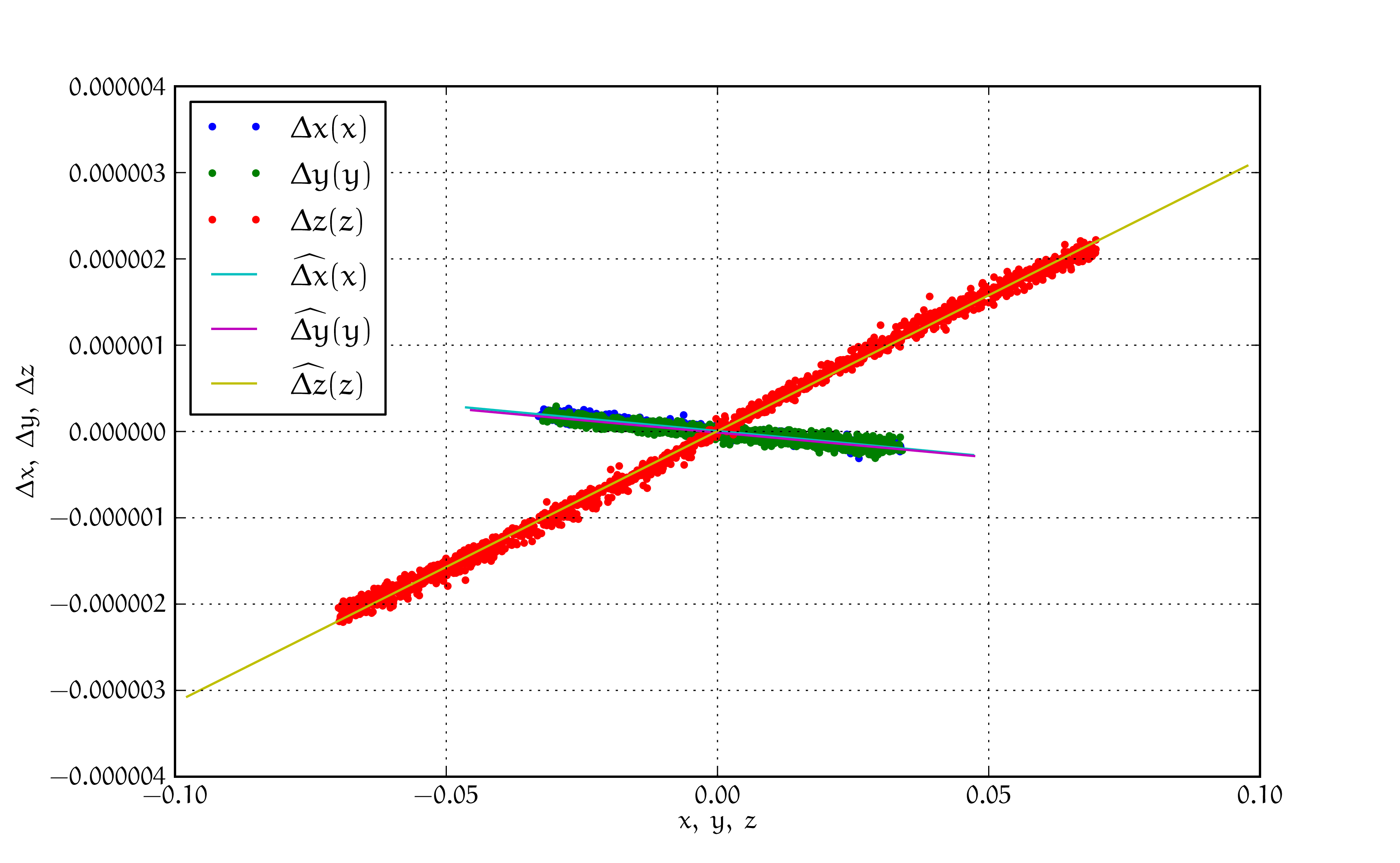

Displacements during uniaxial tension test, plotted against position on respective axis. The slope of the regression $\widehat{\Delta x}(x)$ is the average $\eps_x$ in the specimen. Straining was applied in the direction of the $z$ axis (as $\eps_z>0$) in the case pictured.}

Damage and plasticity parameters

Once the elastic parameters are calibrated, inelastic parameters $\eps_0$, $\eps_f$, $c_{T0}$ and $\phi$ should be adjusted such that we obtain the desired macroscopic properties $f_t$, $f_c$, $G_f$.

The calibration procedure is as follows:

1. We transform model parameters to be dimensionless and material properties to be normalized:

   • parameters

     • $\frac{\eps_f}{\eps_0}$ (relative ductility)

     • $\frac{c_{T0}}{k_T\eps_0}$

     • $\phi$

     • ($\eps_0$ is left as-is)

   • properties

     • $\frac{f_c}{f_t}$ (strength ratio)

     • $\frac{k_N G_f}{f_t^2}$ (characteristic length)

     • ($f_t$ is left as-is)

   There is one additional degree of freedom on both sides ($\eps_0$ and $f_t$), which we will use later.

2. Since there is one additional parameter on the material model side, we fix $c_{T0}$ to a known good value. It was shown that it has the least influence on macroscopic properties, hence the choice.

3. From graphs showing the parameter/property dependence, we set $\eps_f/\eps_0$ to get the desired ${k_N G_f}/{f_t^2}$ (lower right in the figure), since the only remaining parameter $\phi$ has (almost) no influence on ${k_N G_f}/{f_t^2}$ (lower left in the figure).

4. We set $\tan\phi$ such that we obtain the desired $f_c/f_t$ (upper left in the figure).

5. We use the remaining degree of freedom to scale the stress-strain diagram to get the absolute values using radial scaling. By dimensional analysis it can be shown that

$$f_t=k_N\eps_0\Psi\left(\frac{\eps_f}{\eps_0},\frac{c_{T0}}{k_T\eps_0},\phi\right).$$

Since $k_N$ is already determined, it is only $\eps_0$ that will directly determine $f_t$.

Fig. 22 Cross-dependencies of $\eps_0/\eps_f$, $EG_f/f_t^2$ and $\tan\phi$. Since $\tan\phi$ has little influence on $k_N G_f/f_t^2$ (lower left), first $\eps_f/\eps_0$ can be set based on desired $k_N G_f/f_t^2$ (lower right), then $\tan\phi$ is determined so that wanted $f_c/f_t$ ratio is obtained (upper left).

Fig. 23 Radial and vertical scaling of the stress-strain diagram; vertical scaling is used during calibration and is achieved by changing the value of $\eps_0$.

Confinement parameters

Calibrating three confinement-related parameters $\eps_s$, $\tilde K_s$ and $Y_0$ is not algorithmic, but rather a trial-and-error process. On the other hand, typically it will be enough to calibrate the parameters for some generic confinement data, both for the lack of availability of exact measurements and for at best fuzzy matching that can be achieved. The chief reason is that the bilinear relationship for plasticity in compression is far from perfect and could be refined by using a smooth function; in our case, however, the confinement extension was only meant to mitigate high strength overestimation under confinement, not to accurately predict behavior under such conditions. Introducing more complicated functions would further increase the number of parameters, which was not desirable.

The experimental data we use come from [CBavzant00] and [GJ06].

Fig. 24 Confined compression, comparing experimental data and simulation without the confinement extensions of the model. Experimental results (dashed) by Caner.

Consider confined strain-stress diagrams at the preceding figure exhibiting unrealistic behavior under high confinement (-400MPa). Parameters $\eps_s$ and $\tilde K_s$ will influence at which point the curve will get to the hardening branch and what will be its tangent modulus (figure). The $Y_0$ parameter determines evolution of plasticity surface in compression (figure). We recommend the following values of the parameters:

$$\begin{align} \eps_s&=-3\cdot10^{-3}, & \tilde K_s&=0.3, & Y_0&=0.1, \end{align}$$

which give curves in the following figure. It was observed when running multiple simulations that results under high confinement depend greatly on the exact packing configuration, specimen shape and specimen size; therefore, the values given above should be taken with grain of salt.

Fig. 25 Experimental data and simulation in confined compression, using confinement extensions of the model. Cf. [previous figure] for the influence of those extensions.

During simulation, the confinement effect was introduced on the contact level, in the constitutive law itself, as described in Isotropic confinement; the confinement is therefore isotropic and without boundary influence.

Cross-dependencies. Confinement properties may, to certain extent, have influence on inelastic properties. If that happens, reiterating the calibration with new confinement properties should give wanted results quickly.

Rate-dependence parameters

The visco-damage behavior in tension introduced two parameters, characteristic time $\tau_d$ and exponent $M_d$. There is no calibration procedure developed for them, as measuring the response is experimentally challenging and the scatter of results is rather high. Instead, we determined those two parameters by a trial-and-error procedure so that the resulting curve approximately fits the experimental data cloud − we use figures from [RG03], which are in turn based on published experiments.

The resulting curves show tension and compression. Because DEM computation would be very slow (large number of steps, determined by critical timestep) for slow rates, those results were computed with the same model implemented in the OOFEM framework (using a static implicit FEM model); this also served to verify that both implementations give identical results. For high loading rates, DEM results deviate, since there is inertial mass that begins to play an important role.

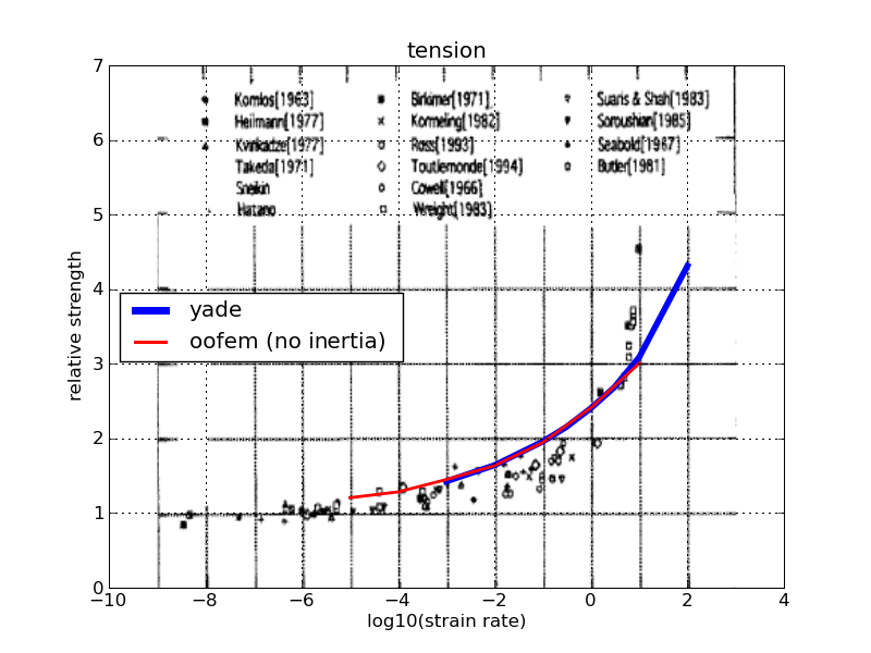
Fig. 26 Experimental data and simulation results for tension.

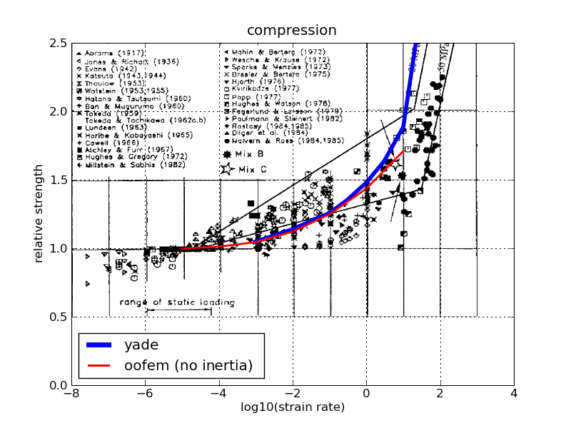
Fig. 27 Experimental data and simulation results for compression.

The values that we recommend to use are

$$\begin{align} \tau_d&=1000\,{\rm s}, \\ M_d&=0.3. \end{align}$$

Calibration of visco-plastic parameters was rather simple: we found out that it has no beneficial effect on results; therefore, visco-plasticity should be deactivated. In the implementation, this is done by setting $\tau_{pl}$ (ConcretePhys.plTau to an arbitrary non-positive value).

Tip

Report issues or inclarities to github.