Basics
Overview
This chapter explains how to write script for a very simple DEM simulation (a sphere falling onto plane) and how to run it. It clarifies the function of particles, nodes and engines.
Scene
The whole simulation is contained in a single woo.core.Scene object, which contains the rest; a scene can be loaded from and saved to a file, just like any other object. Scene defines things like timestep (dt) or periodic boundary conditions (cell).
It also contains several fields; each field is dedicated to a one simulation method, and the fields can be semi-independent. As we go for a DEM simulation, the important field for us is a DemField; that is the one containing particles and contacts (we deal with that later); we can also define gravity acceleration for this field by setting DemField.gravity.
There can be an unlimited number of scenes, each of them independent of others. Only one can be controlled by the UI (and shown in the 3d view); it is the one assigned to woo.master.scene, the master scene object.
New scene with the DEM field can be initialized in this way:
import woo, woo.core, woo.dem   # import modules we use
S=woo.core.Scene()              # create the scene object
f=woo.dem.DemField()            # create the field object
f.gravity=(0,0,-9.81)           # set gravity acceleration
S.fields=[f]                     # add field to the scene
woo.master.scene=S              # this will be the master scene now
Since all objects can take keyword arguments when constructed, and assignments can be chained in Python, this can be written in a much more compact way:
Woo[1]: S=woo.master.scene=woo.core.Scene(fields=[woo.dem.DemField(gravity=(0,0,-9.81))])
The DEM field can be accessed as S.fields[0], but this is not very convenient. There is a shorthand defined, S.dem, which always returns the (first) DEM field attached to the scene object.
Woo[2]: S.fields[0]
Out[2]: <DemField @ 0x3eb2b40>

Woo[3]: S.dem
Out[3]: <DemField @ 0x3eb2b40>

Woo[4]: S.dem.gravity
Out[4]: Vector3(0,0,-9.81)
Particles
Particles are held in the DemField.par container (shorthand for DemField.particles); new particles can be added using the add method.
Particles are not simple objects; they hold together material and shape (the geometry – such as Sphere, Capsule, Wall, …) and other thigs. Shape is attached to one (for mononodal particles, like spheres) or several (for multinodal particles, like facets) nodes with some position and orientation, each node holds DemData containing mass, inertia, velocity and so on.
To avoid complexity, there are utility functions that take a few input data and return a finished Particle.
We can define an infinite plane (Wall) in the \(xy\)-plane with \(z=0\) and add it to the scene:
wall=woo.dem.Wall.make(0,axis=2)
S.dem.par.add(wall)
Walls are fixed by default, and the woo.utils.defaultMaterial was used as material – the default material is not good for real simulations, but it is handy for quick demos. We also define a sphere and put it in the space above the wall:
sphere=woo.dem.Sphere.make((0,0,2),radius=.2)
S.dem.par.add(sphere)
The add method can also take several particles as list, so we can add both particles in a compact way:
S.dem.par.add([
   woo.dem.Wall.make(0,axis=2),
   woo.dem.Sphere.make((0,0,2),radius=.2)
])
or in one line:
Woo[5]: S.dem.par.add([woo.dem.Wall.make(0,axis=2),woo.dem.Sphere.make((0,0,2),radius=.2)])
Out[5]: [0, 1]

Woo[6]: S.dem.par[0]
Out[6]: <Particle #0 [Wall] @ 0x167afb0>

Woo[7]: S.dem.par[1]
Out[7]: <Particle #1 [Sphere] @ 0x23d0c80>
Besides creating the particles, it must also be said which nodes we actually want to have moving, i.e. subject to motion integration. add tries to be smart by default, and only adds particles which have non-zero mass (Wall does not, as created by default) or velocity or something else (see add and guessMoving if you want to know more).
Let’s check what was done:
Woo[8]: len(S.dem.par),len(S.dem.nodes)
Out[8]: (2, 1)

Woo[9]: list(S.dem.nodes)
Out[9]: [<Node @ 0x2dcd650, at (0,0,2)>]
Engines
After adding particles to the scene, we need to tell Woo what to do with those particles. Scene.engines describe things to do. Engines are run one after another; once the sequence finishes, time is incremented by dt, step is incremented by one, and the sequence starts over.
Although the engine sequence can get complex, there is a pre-cooked engine sequence DemField.minimalEngines suitable for most scenarios; it consists of the minimum of what virtually every DEM simulation needs:
motion integration (compute accelerations from contact forces and gravity on nodes, update velocities and positions);
collision detection (find particle overlaps)
contact resolution (compute forces resulting from overlaps; without any other parameters, the linear contact model is used);
automatic time-step adjustment based on numerical stability criteria (not strictly necessary, but highly useful)
Assigning the engines is simple (in simple simulations):
Woo[10]: S.engines=S.dem.minimalEngines(damping=.2)
Notice that we passed the damping parameter, which is necessary for models without internal dissipation; more on this later.
Periodic engines
Engines usually run at every time-step once. Some (deriving from woo.core.PeriodicEngine) run with a different periodicity, which can be specified using stepPeriod (run every \(N\) steps), virtPeriod (run every \(x\) seconds of the in-simulation, “virtual” time), realPeriod (run every \(x\) seconds of the human time).
The number of the engine being run can be limited via nDo; the number of how many times it was run is stored in nDone.
Woo[11]: d=S.engines[-1]   # last engine

Woo[12]: d.stepPeriod      # how often this engine runs
Out[12]: 100

Woo[13]: S.run(500,True)   # run 500 steps -- see below for explanation

Woo[14]: d.nDone           # how many times the engine was run
Out[14]: 5
One of the most flexible engines is woo.core.PyRunner which allows one to run arbitrary python code (given as string); we can use it here to print simulation time, just as an example
Woo[15]: S
Out[15]: <Scene @ 0x42ffe80>

Woo[16]: S.engines=S.engines+[woo.core.PyRunner(100,'print(S.step,S.time,S.dt)')]

Woo[17]: S.run(500,True)
0 0.0 0.0018000000000000002
100 0.1799999999999998 0.0018000000000000002
200 0.3600000000000011 0.0018000000000000002
300 0.5400000000000035 0.0018000000000000002
400 0.7200000000000059 0.0018000000000000002
Extras
Two handy things to do before we run the simulation:
Limit the simulation speed; this is never used for big simulations, but now we want to see things as they happen. We can insert a small pause after each step (here we use 5ms):
Woo[18]: S.throttle=5e-3
Save the simulation so that we can quickly reload it using the ↻ (reload) button:
Woo[19]: S.saveTmp()
The woo.core.Object.saveTmp function saves to the memory, so everything will be lost when Woo finishes, but that is just fine now.
Running
All in all, the minimal simulation of a sphere falling onto plane looks like this:
Note
To avoid typing woo.dem all the time, the module woo.dem was imported as from woo.dem import *; the same could be also done with the woo.core module.
import woo
from woo.dem import *
from woo.core import *
# scene:
S=woo.master.scene=woo.core.Scene(fields=[DemField(gravity=(0,0,-9.81))])
# particles:
S.dem.par.add(Wall.make(0,axis=2),nodes=False)
S.dem.par.add(Sphere.make((0,0,2),radius=.2))
# engines:
S.engines=S.dem.minimalEngines(damping=.2)
# extras:
S.throttle=0.005
S.saveTmp()
Save this to a file, name it e.g. basic-1.py (or whatever ending with .py, which is the extension indicating Python) and run woo from the terminal, passing the basic-1.py as argument to Woo. You must run Woo from the same directory as where the script is located (by default, new terminal opens in your home directory; if the basic-1.py is saved for example under ~/Documents, you have to type cd Documents first):
woo basic-1.py
You should see something similar to this:
Welcome to Woo /r3484
Running script basic-1.py
[[ ^L clears screen, ^U kills line. F12 controller, F11 3d view, F10 both, F9 generator, F8 plot. ]]
Woo [1]:
and the controller window opens. The script was executed, but the simulation is not yet running – the script does not ask for that. Click on the 3D button to look at the scene and something like this appears:
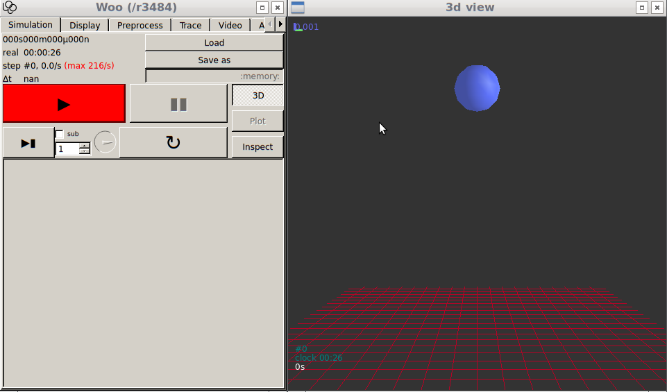
Fig. 3 User interface after running the basic-1.py script.
When you click the ▶ (play) button , you will see the simulation running:
The ▶ button is red as we set S.throttle; you can change the value using the dial under ▶. Try also clicking ▮▮ (pause), ▶▮ (single step, or several steps as set next to it) and ↻ (that will load the state when you said S.saveTmp()). The controller shows some basic data, some of which are also presented in the corner of the 3d view: time, step number, timestep.
Clicking the Inspector button will present internal structure of the simulation – particles, engines, contacts (there will be no contact most the time, in this simulation). You can select a particle with by Shift-click on the particle in the 3d view; it will be selected in the inspector as well.
The simulation can also be run from the script or the command line in terminal:
Woo[20]: S.one()         # one step, like ▶▮

Woo[21]: S.run()         # run in background until stopped, like ▶

Woo[22]: S.stop()        # stop the simulation (does nothing if not running), like ▮▮

# where are we at now?
Woo[23]: S.step, S.time, S.dt
Out[23]: (2, 0.0036000000000000003, 0.0018000000000000002)

Woo[24]: S.run(200)      # run 200 steps in background

Woo[25]: S.wait()        # wait for the background to finish, then return
Warning
When the script is executed, it defines the S variable to point to your scene. When the scene is reloaded via ↻ (which invokes woo.master.reload), woo.master.scene refers to the newly loaded scene, but S is still pointing to the old object:
Woo[26]: import woo; S=woo.master.scene; S.dt=1e-9; S.saveTmp()

Woo[27]: S, woo.master.scene      ## both point to the same scene -- look at the address
Out[27]: (<Scene @ 0x2cdd2c0>, <Scene @ 0x2cdd2c0>)

Woo[28]: woo.master.reload()      ## reload the master scene
Out[28]: <Scene @ 0x3ec9df0>

Woo[29]: S, woo.master.scene      ## two different scenes
Out[29]: (<Scene @ 0x2cdd2c0>, <Scene @ 0x3ec9df0>)

Woo[30]: S.one()                  ## will run the OLD scene, but it won't be seen graphically :|

Woo[31]: S=woo.master.scene       ## set S to the "good" value after reloading

Woo[32]: S.one()                  ## runs the current master scene, OK :)
All data in the scene can be accessed as well:
Woo[1]: from woo.dem import *; from woo.core import *; import woo; S=Scene(fields=[DemField(gravity=(0,0,-9.81),par=[Wall.make(0,axis=2),Sphere.make((0,0,.2),.2)])],engines=DemField.minimalEngines(damping=.2)); S.run(100,True)

Woo[2]: S.dem                    # the DEM field
Out[2]: <DemField @ 0x3e306a0>

Woo[3]: S.dem.gravity=(0,0,-20)  # set different gravity acceleration

Woo[4]: S.step                   # step number
Out[4]: 100

Woo[5]: S.dt                     # time-step
Out[5]: 0.0018000000000000002

Woo[6]: S.engines                # all engines
Out[6]:
[<Leapfrog @ 0x3e8df90>,
 <InsertionSortCollider @ 0x3e13b90>,
 <ContactLoop @ 0x3e8e260>,
 <DynDt @ 0x2dde280>]

Woo[7]: S.dem.par[0]             # first particle (numbering starts from 0)
Out[7]: <Particle #0 [Wall] @ 0x37430b0>

Woo[8]: S.dem.par[1]             # second particle
Out[8]: <Particle #1 [Sphere] @ 0x39652d0>

Woo[9]: S.dem.par[-1]            # last particle; negative numbers from the end
Out[9]: <Particle #1 [Sphere] @ 0x39652d0>

Woo[10]: p1=S.dem.par[1]

Woo[11]: p1.pos                   # position of particle #1
Out[11]: Vector3(0,0,0.19989534871327705)

Woo[12]: p1.shape                 # geometrical shape of particle #1
Out[12]: <Sphere r=0.200000 @ 0x42dff80>

Woo[13]: p1.f                     # force on the particle (only works for uninodal particles)
Out[13]: Vector3(0,0,0.035458285940762835)

Woo[14]: p1.t                     # torque on the particle (uninodal only)
Out[14]: Vector3(0,0,0)

Woo[15]: p1.contacts              # contacts of this particle (*real* contacts only), as mapping of id and contact object
Out[15]: {0: <Contact ##0+1 @ 0x7fba04002370>}

Woo[16]: p1.con                   # ids of contacting particles (shorthand for keys of p1.contacts)
Out[16]: [0]

Woo[17]: p1.tacts                 # contact objects (shorthand for values of p1.contacts)
Out[17]: [<Contact ##0+1 @ 0x7fba04002370>]

Woo[18]: len(p1.con)              # number of contacts of this particle
Out[18]: 1

Woo[19]: p1.contacts[0]           # contact between 0 and 1
Out[19]: <Contact ##0+1 @ 0x7fba04002370>

Woo[20]: S.dem.con[0,1]           # the same contact, accessed differently
Out[20]: <Contact ##0+1 @ 0x7fba04002370>

Woo[21]: c01=S.dem.con[0,1]

Woo[22]: c01.geom                 # contact geometry
Out[22]: <L6Geom @ 0x7fb9f8000b70>

Woo[23]: c01.geom.uN              # normal overlap
Out[23]: -0.00010465128672296209

Woo[24]: c01.phys.force           # force in contact-local coordinates
Out[24]: Vector3(-328.7717135575768,0,0)
Tip
Report issues or inclarities to github.